Regression Based Approach for Motif Selection
Dania Machlab, Lukas Burger, Charlotte Soneson, Michael Stadler
2026-01-27
Source:vignettes/selecting_motifs_with_randLassoStabSel.Rmd
selecting_motifs_with_randLassoStabSel.Rmd
Introduction
Identifying important transcription factor (TF) motifs, as shown in
the
main vignette, could also be done using a regression-based approach,
where motifs have to compete against each other for selection. In this
framework, the response vector can be the observed experimental measure
of interest, e.g. log-fold changes of accessibility for a set of
regions, and the predictors consist of the TF motif hits across those
regions. In monaLisa,
we implement the randomized lasso stability selection proposed by Meinshausen and Bühlmann (2010) with the
improved error bounds introduced by Shah and
Samworth (2013). We have modified the
stabs::glmnet.lasso function used by
stabs::stabsel from the stabs package
to implement the randomized lasso.
Lasso stability selection performs the lasso regression multiple times on subsamples of the data, and returns a selection probability for each predictor (number of times selected divided by number of regressions done). With the randomized lasso, a weakness parameter is additionally used to vary the lasso penalty term to a randomly chosen value between [, /weakness] for each predictor. This type of regularization has advantages in cases where the number of predictors exceeds the number of observations, in selecting variables consistently, demonstrating better error control and not depending strongly on the penalization parameter (Meinshausen and Bühlmann 2010).
With this approach, TF motifs compete against each other to explain the response vector, and we can also include additional predictors like GC content to compete against the TF motifs for selection. This is especially useful if the response is biased by sequence composition, for example if regions with higher GC content tend to have higher response values.
It is worth noting that, as with any regression analysis, the interpretability of the results depends strongly on the quality of the predictors. Hence, increasing the size of the motif database is not, in itself, a guarantee for more interpretable results, since the added motifs may be unrelated to the signal of interest. In addition, as discussed in section @ref(collinearity), a high level of redundancy, resulting in strong correlations among the motifs, may result in more ambiguous selection probabilities in the regression approach. In fact, also for the binned approach, although the motifs are evaluated independently for association with the outcome, a high degree of redundancy can lead to large collections of very similar motifs showing significant enrichments, complicating interpretability of the results.
Motif selection with Randomized Lasso Stability Selection
In the example below, we select for TF motifs explaining log-fold changes in chromatin accessibility (ATAC-seq) across the enhancers between mouse liver and lung tissue at P0, but this can be applied to other data types as well (ChIP-seq, RNA-seq, methylation etc.). Positive log2-fold changes indicate more accessibility in the liver tissue, whereas negative values indicate more accessibility in the lung tissue.
Load packages
We start by loading the needed packages:
library(monaLisa)
library(JASPAR2020)
library(TFBSTools)
library(BSgenome.Mmusculus.UCSC.mm10)
library(Biostrings)
library(SummarizedExperiment)
library(ComplexHeatmap)
library(circlize)
library(ggrepel)
Load dataset
In this example dataset from ENCODE (The ENCODE Project Consortium 2012), and available in monaLisa, we have quantified ATAC-seq reads on enhancers in mouse P0 lung and liver tissues. The log2-fold change (our response vector in this example) is for liver vs lung chromatin accessibility. We are using a set of 10,000 randomly sampled enhancers to illustrate how randomized lasso stability selection can be used to select TF motifs.
# load GRanges object with logFC and peaks
gr_path <- system.file("extdata", "atac_liver_vs_lung.rds",
                       package = "monaLisa")
gr <- readRDS(gr_path)
Get TFBS per motif and peak
We will now construct the transcription factor binding site (TFBS)
matrix for known motifs (from a database like JASPAR2020)
in the given peak regions. We use the findMotifHits
function to scan for TF motif hits. This matrix will be the predictor
matrix in our regression. This step may take a while, and it may be
useful to parallelize it using the BPPARAM argument (e.g.
to run on n parallel threads using the multi-core backend,
you can use:
findMotifHits(..., BPPARAM = BiocParallel::MulticoreParam(n))).
As mentioned, this framework offers the flexibility to add additional predictors to compete against the TF motifs for selection. Here, we add the fraction of G+C and CpG observed/expected ratio as predictors, to ensure that selected TF motifs are not just detecting a simple trend in GC or CpG composition.
# get PFMs (vertebrate TFs from Jaspar)
pfms <- getMatrixSet(JASPAR2020, list(matrixtype = "PFM",
                                      tax_group = "vertebrates"))

# randomly sample 300 PFMs for illustration purposes (for quick runtime)
set.seed(4563)
pfms <- pfms[sample(length(pfms), size = 300)]

# convert PFMs to PWMs
pwms <- toPWM(pfms)

# get TFBS on given GRanges (peaks)
# suppress warnings generated by matchPWM due to the presence of Ns
# in the sequences
peakSeq <- getSeq(BSgenome.Mmusculus.UCSC.mm10, gr)
suppressWarnings({
  hits <- findMotifHits(query = pwms, subject = peakSeq, min.score = 10.0,
                        BPPARAM = BiocParallel::SerialParam())
})

# get TFBS matrix
TFBSmatrix <- unclass(table(factor(seqnames(hits), levels = seqlevels(hits)),
                            factor(hits$pwmname, levels = name(pwms))))
TFBSmatrix[1:6, 1:6]
#>
#>               NR3C2 Arnt LHX1 SNAI1 MAFG ZSCAN4
#>   peak_51663      0    0    0     0    0      0
#>   peak_57870      0    0    0     0    0      0
#>   peak_2986       2    0    0     0    0      0
#>   peak_124022     0    0    0     0    0      0
#>   peak_29925      0    2    0     1    0      0
#>   peak_95246      0    0    0     0    0      0

# remove TF motifs with 0 binding sites in all regions
zero_TF <- colSums(TFBSmatrix) == 0
sum(zero_TF)
#> [1] 2
TFBSmatrix <- TFBSmatrix[, !zero_TF]

# calculate G+C and CpG obs/expected
fMono <- oligonucleotideFrequency(peakSeq, width = 1L, as.prob = TRUE)
fDi <- oligonucleotideFrequency(peakSeq, width = 2L, as.prob = TRUE)
fracGC <- fMono[, "G"] + fMono[, "C"]
oeCpG <- (fDi[, "CG"] + 0.01) / (fMono[, "G"] * fMono[, "C"] + 0.01)

# add GC and oeCpG to predictor matrix
TFBSmatrix <- cbind(fracGC, oeCpG, TFBSmatrix)
TFBSmatrix[1:6, 1:6]
#>                fracGC     oeCpG NR3C2 Arnt LHX1 SNAI1
#> peak_51663  0.5155709 0.4079115     0    0    0     0
#> peak_57870  0.4963235 0.3048298     0    0    0     0
#> peak_2986   0.4008264 0.3103806     2    0    0     0
#> peak_124022 0.4572650 0.4429813     0    0    0     0
#> peak_29925  0.4675000 0.3495939     0    2    0     1
#> peak_95246  0.5144509 0.4020976     0    0    0     0
A note on collinearity
At this point it is useful for the user to get an overall feeling of the collinearity structure in the TFBS matrix. Motifs that share a lot of similar binding sites across the peaks will be highly correlated. High collinearity between predictors is a well known problem in linear regression. It particularly manifests itself in the lasso regression for example, where if variables are equally highly correlated with the response, not all are co-selected as predictors (if they are signal variables). Instead, one is arbitrarily chosen while the others’ coefficients are set to zero. The rationale is that the non-selected correlated predictors do not provide much additional information to explain the response. It is good to be aware of these properties of regression, and to place more weight on the meaning of the selected motif itself, rather than the specific TF name when interpreting the results.
If many cases of high correlations exist and this is a concern, one may consider selecting a representative set of predictors to use. This may for example be achieved by clustering the weight matrices beforehand and using only one representative motif per cluster for running the regression, using tools such as for example RSAT (Castro-Mondragon et al. 2017). RSAT-derived clusters of Jaspar weight matrices can be found at https://jaspar.genereg.net/matrix-clusters/vertebrates/.
If the user is interested in working with all correlated motifs, the binned approach is preferable as the motifs are independently tested for significance (see the binned enrichment vignette). In the regression-based approach on the other hand, we can more clearly understand the relative contributions of TF motifs to the response in the context of each other.
Identify important TFs
We can now run randomized lasso stability selection to identify TFs
that are likely to explain the log-fold changes in accessibility. The
exact choice of parameter values for this approach will depend largely
on how stringent the user wishes to be and how much signal there is in
the data. For example, for more stringent selections, one may decrease
the value of the weakness parameter which will make it
harder for a variable to get selected. The user is in control of false
discoveries with the PFER parameter, which indicates the
number of falsely selected variables. As for the selection probability
cutoff, Meinshausen and Bühlmann (2010)
argue that values in the range of [0.6, 0.9] should give similar
results. See the randLassoStabSel function for more details
and default parameter values as well as the stabs::stabsel
function for the default assumptions on the stability selection
implementation by Shah and Samworth
(2013).
## randLassoStabSel() is stochastic, so if we run with parallelization
##   (`mc.cores` argument), we must select a random number generator that can
##   provide multiple streams of random numbers used in the `parallel` package
##   and set its seed for reproducible results
# RNGkind("L'Ecuyer-CMRG")
# set.seed(123)
# se <- randLassoStabSel(x = TFBSmatrix, y = gr$logFC_liver_vs_lung,
#                        cutoff = 0.8, mc.preschedule = TRUE,
#                        mc.set.seed = TRUE, mc.cores = 2L)

# if not running in parallel mode, it is enough to use set.seed() before
#   the call to ensure reproducibility (`mc.sores = 1`)
set.seed(123)
se <- randLassoStabSel(x = TFBSmatrix, y = gr$logFC_liver_vs_lung,
                       cutoff = 0.8)
se
#> class: SummarizedExperiment
#> dim: 10000 300
#> metadata(12): stabsel.params.cutoff stabsel.params.selected ...
#>   stabsel.params.call randStabsel.params.weakness
#> assays(1): x
#> rownames(10000): peak_51663 peak_57870 ... peak_98880 peak_67984
#> rowData names(1): y
#> colnames(300): fracGC oeCpG ... CLOCK OLIG2
#> colData names(20): selProb selected ... regStep16 regStep17

# selected TFs
colnames(se)[se$selected]
#>  [1] "NKX2-5"       "GATA1::TAL1"  "HNF1B"        "HNF4A(var.2)" "Nr2f6"
#>  [6] "ONECUT3"      "MYF5"         "THRB"         "ISL2"         "NR2C2"
#> [11] "TEAD3"        "TEAD4"        "GATA3"        "RORA"         "NFIC"
#> [16] "ZEB1"
The stability paths visualize how predictors get selected over decreasing regularization stringency (from left to right):
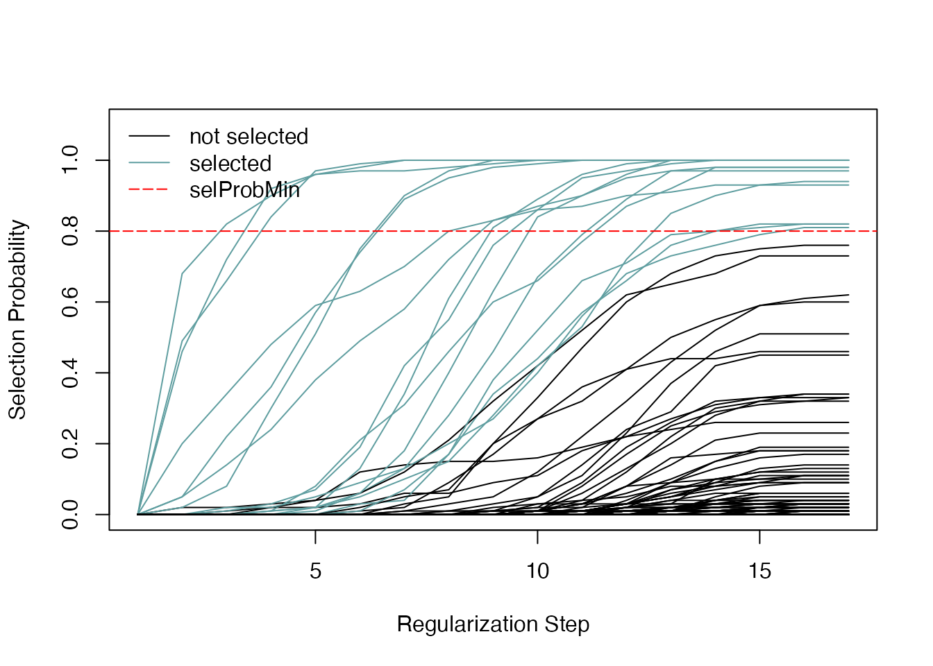
Each line corresponds to a predictor, and we can see the selection probabilities as a function of the regularization steps, corresponding to decreasing values for the lambda regularization parameter in lasso. The predictor (TF motif) selection happens at the last step, given the specified minimum probability.
We can additionally show the labels of the predictors which were selected. Note that if predictors have the same y-value at the last regularization step, they are shown in a random order. To reproduce the plot, you will need to set a seed.
set.seed(123)
plotStabilityPaths(se, labelPaths = TRUE)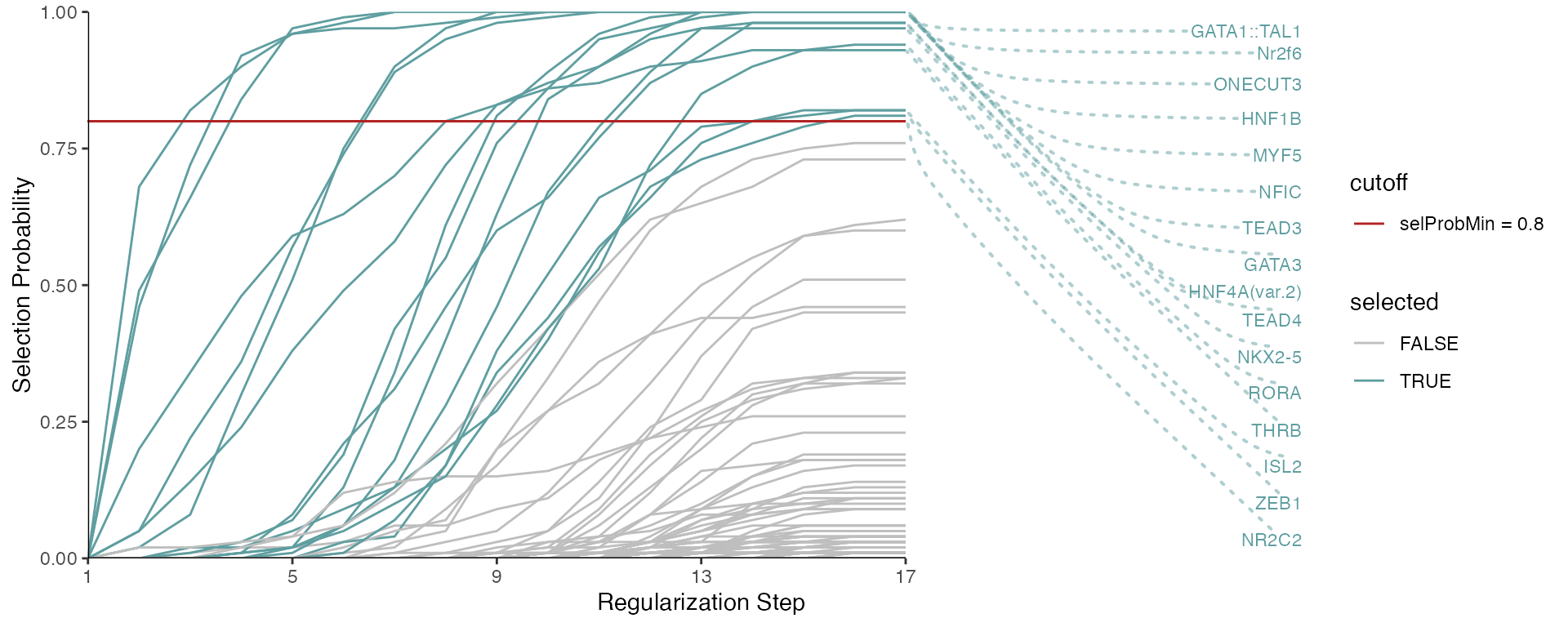
Alternatively, we can visualize specific predictors, regardless of whether or not they were selected.
set.seed(123)
plotStabilityPaths(se, labelPaths = TRUE, labelNudgeX = 3,
                   labels = c("ISL2", "NR2C2", "NR2F1", "GATA4"))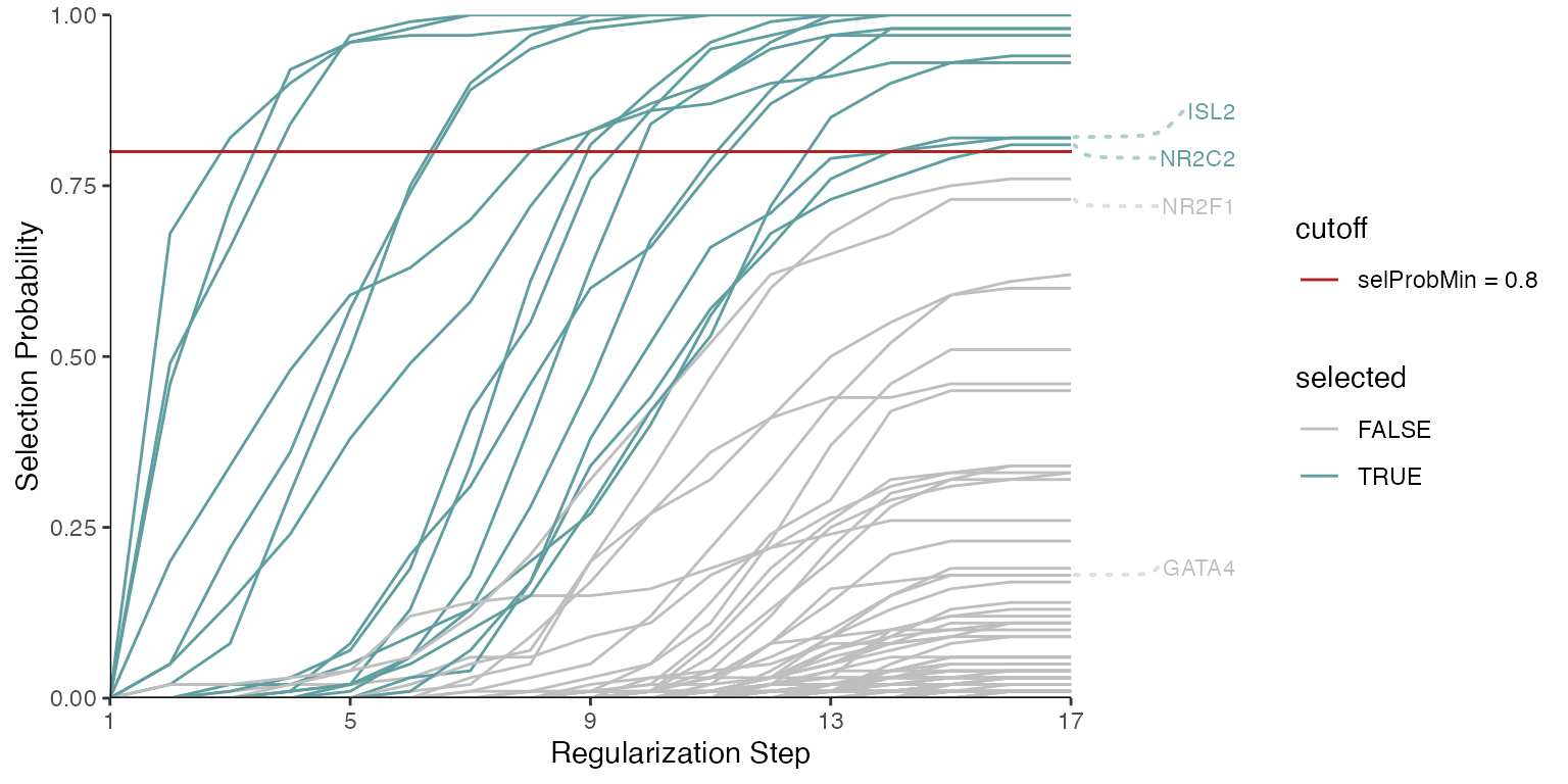
We can also visualize the selection probabilities of the selected TF
motifs, optionally multiplied by the sign of the correlation to the
response vector, to know how the TF relates to the change of
accessibility (directional parameter). In our example,
positive correlations to the response vector indicate a correlation with
enhancers more accessible in the liver, whereas negative ones indicate a
correlation with enhancers more accessible in the lung. Note that
although one can vary the selProbMinPlot argument which
sets the selection probability cutoff, it is best to re-run randomized
lasso stability selection with the new cutoff, as this influences other
parameter choices the model uses internally. See Meinshausen and Bühlmann (2010) for more
details.
plotSelectionProb(se, directional = TRUE, ylimext = 0.5)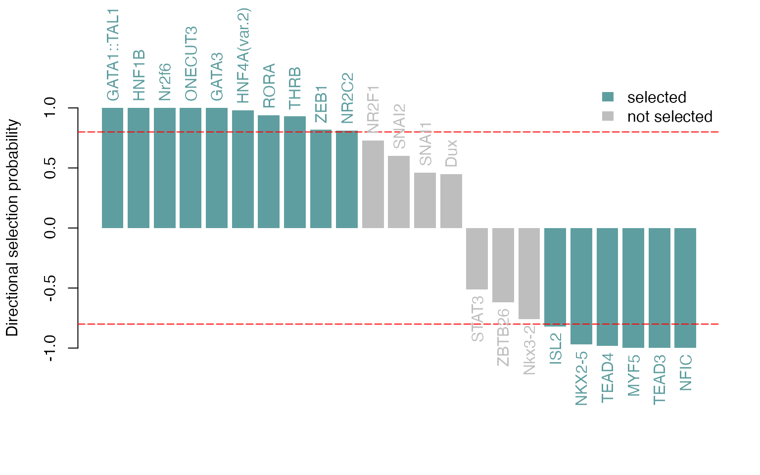
Next, we visualize the correlation structure of the selected TF motifs within the TFBS matrix. While the collinearity of predictors is a general issue in regression-based approaches, randomized lasso stability selection normally does better at co-selecting intermediately correlated predictors. In practice, we see it select predictors with correlations as high as 0.9. However, it is good to keep in mind that this can be an issue, and that predictors that are highly correlated with each other might not end up being co-selected (see section @ref(collinearity)).
# subset the selected TFs
sel <- colnames(se)[se$selected]
se_sub <- se[, sel]

# exclude oeCpG and fracGC
excl <- colnames(se_sub) %in% c("oeCpG", "fracGC")
se_sub <- se_sub[, !excl]

# correlation matrix
TFBSmatrixCorSel <- cor(TFBSmatrix[, colnames(se_sub)], method = "pearson")

# heatmap
pfmsSel <- pfms[match(colnames(TFBSmatrixCorSel), name(pfms))]
maxwidth <- max(sapply(TFBSTools::Matrix(pfmsSel), ncol))
seqlogoGrobs <- lapply(pfmsSel, seqLogoGrob, xmax = maxwidth)

hmSeqlogo <- rowAnnotation(logo = annoSeqlogo(seqlogoGrobs, which = "row"),
                           annotation_width = unit(2, "inch"),
                           show_annotation_name = FALSE
)

colAnn <- HeatmapAnnotation(AUC = se_sub$selAUC, selProb = se_sub$selProb,
                            show_legend = TRUE,
                            show_annotation_name = TRUE,
                            col = list(
                              AUC = colorRamp2(c(0, 1),
                                               c("white", "brown")),
                              selProb = colorRamp2(c(0, 1),
                                                   c("white", "steelblue")))
)

Heatmap(TFBSmatrixCorSel,
        show_row_names = TRUE,
        show_column_names = TRUE,
        name = "Pear. Cor.", column_title = "Selected TFs",
        col = colorRamp2(c(-1, 0, 1), c("blue", "white", "red")),
        right_annotation = hmSeqlogo,
        top_annotation = colAnn)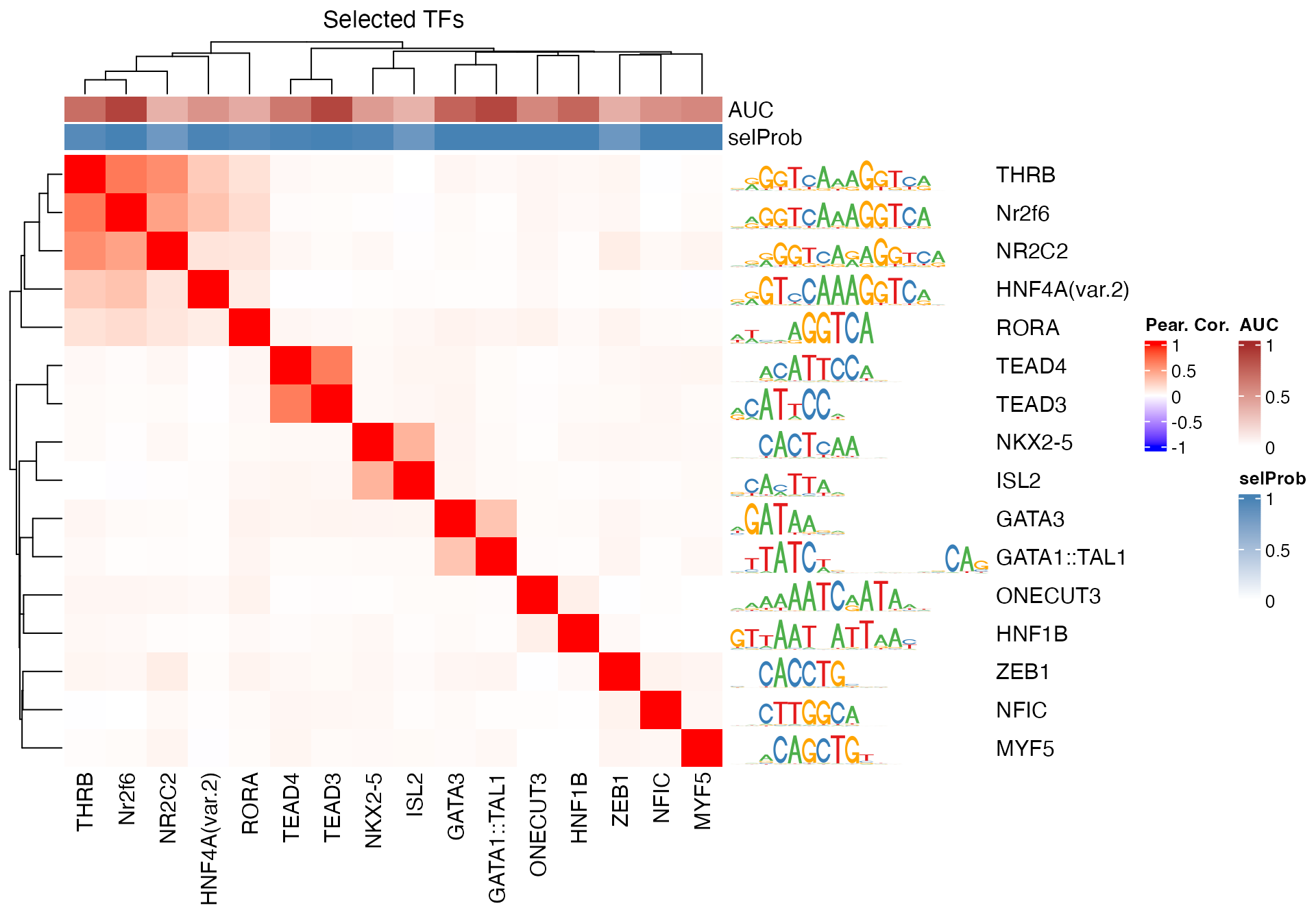
We can examine the peaks that have hits for a selected TF motif of interest, ordered by absolute accessibility changes.
TF <- sel[2]
TF
#> [1] "GATA1::TAL1"

i <- which(assay(se, "x")[, TF] > 0) # peaks that contain TF hits...
nm <- names(sort(abs(gr$logFC_liver_vs_lung[i]),
                 decreasing = TRUE)) # ... order by |logFC|

gr[nm]
#> GRanges object with 1102 ranges and 1 metadata column:
#>               seqnames              ranges strand | logFC_liver_vs_lung
#>                  <Rle>           <IRanges>  <Rle> |           <numeric>
#>    peak_59642     chr8   80499941-80501128      * |             5.31505
#>    peak_58095     chr8   40658907-40659590      * |             5.13536
#>   peak_100144    chr14   69318236-69318909      * |             5.09810
#>    peak_98635    chr14   41124351-41126121      * |             5.07972
#>    peak_42826     chr6   29700952-29701570      * |             5.02324
#>           ...      ...                 ...    ... .                 ...
#>    peak_45104     chr6   84095148-84095495      * |        -0.020828315
#>    peak_16029     chr2 132269993-132270884      * |         0.007621169
#>    peak_55106     chr7 129526059-129526291      * |         0.004120784
#>    peak_97436    chr14   20873345-20873654      * |         0.000765027
#>    peak_67068     chr9   75050089-75050395      * |        -0.000217812
#>   -------
#>   seqinfo: 19 sequences from an unspecified genome; no seqlengths
Session info and logo
The monaLisa logo uses a drawing that was obtained from http://vectorish.com/lisa-simpson.html under the Creative Commons attribution - non-commercial 3.0 license: https://creativecommons.org/licenses/by-nc/3.0/.
This vignette was built using:
sessionInfo()
#> R Under development (unstable) (2026-01-26 r89334)
#> Platform: aarch64-apple-darwin20
#> Running under: macOS Sequoia 15.7.3
#>
#> Matrix products: default
#> BLAS:   /System/Library/Frameworks/Accelerate.framework/Versions/A/Frameworks/vecLib.framework/Versions/A/libBLAS.dylib
#> LAPACK: /Library/Frameworks/R.framework/Versions/4.6-arm64/Resources/lib/libRlapack.dylib;  LAPACK version 3.12.1
#>
#> locale:
#> [1] en_US.UTF-8/en_US.UTF-8/en_US.UTF-8/C/en_US.UTF-8/en_US.UTF-8
#>
#> time zone: UTC
#> tzcode source: internal
#>
#> attached base packages:
#> [1] grid      stats4    stats     graphics  grDevices utils     datasets
#> [8] methods   base
#>
#> other attached packages:
#>  [1] ggrepel_0.9.6                      ggplot2_4.0.1
#>  [3] circlize_0.4.17                    ComplexHeatmap_2.27.0
#>  [5] SummarizedExperiment_1.41.0        Biobase_2.71.0
#>  [7] MatrixGenerics_1.23.0              matrixStats_1.5.0
#>  [9] BSgenome.Mmusculus.UCSC.mm10_1.4.3 BSgenome_1.79.1
#> [11] rtracklayer_1.71.3                 BiocIO_1.21.0
#> [13] Biostrings_2.79.4                  XVector_0.51.0
#> [15] GenomicRanges_1.63.1               Seqinfo_1.1.0
#> [17] IRanges_2.45.0                     S4Vectors_0.49.0
#> [19] BiocGenerics_0.57.0                generics_0.1.4
#> [21] TFBSTools_1.49.0                   JASPAR2020_0.99.10
#> [23] monaLisa_1.17.1                    BiocStyle_2.39.0
#>
#> loaded via a namespace (and not attached):
#>  [1] DBI_1.2.3                   bitops_1.0-9
#>  [3] stabs_0.6-4                 rlang_1.1.7
#>  [5] magrittr_2.0.4              clue_0.3-66
#>  [7] GetoptLong_1.1.0            compiler_4.6.0
#>  [9] RSQLite_2.4.5               png_0.1-8
#> [11] systemfonts_1.3.1           vctrs_0.7.1
#> [13] pwalign_1.7.0               pkgconfig_2.0.3
#> [15] shape_1.4.6.1               crayon_1.5.3
#> [17] fastmap_1.2.0               labeling_0.4.3
#> [19] caTools_1.18.3              Rsamtools_2.27.0
#> [21] rmarkdown_2.30              ragg_1.5.0
#> [23] DirichletMultinomial_1.53.0 purrr_1.2.1
#> [25] bit_4.6.0                   xfun_0.56
#> [27] glmnet_4.1-10               cachem_1.1.0
#> [29] cigarillo_1.1.0             jsonlite_2.0.0
#> [31] blob_1.3.0                  DelayedArray_0.37.0
#> [33] BiocParallel_1.45.0         parallel_4.6.0
#> [35] cluster_2.1.8.1             R6_2.6.1
#> [37] bslib_0.10.0                RColorBrewer_1.1-3
#> [39] jquerylib_0.1.4             Rcpp_1.1.1
#> [41] bookdown_0.46               iterators_1.0.14
#> [43] knitr_1.51                  Matrix_1.7-4
#> [45] splines_4.6.0               tidyselect_1.2.1
#> [47] abind_1.4-8                 yaml_2.3.12
#> [49] doParallel_1.0.17           codetools_0.2-20
#> [51] curl_7.0.0                  lattice_0.22-7
#> [53] tibble_3.3.1                withr_3.0.2
#> [55] S7_0.2.1                    evaluate_1.0.5
#> [57] desc_1.4.3                  survival_3.8-6
#> [59] pillar_1.11.1               BiocManager_1.30.27
#> [61] foreach_1.5.2               RCurl_1.98-1.17
#> [63] scales_1.4.0                gtools_3.9.5
#> [65] glue_1.8.0                  seqLogo_1.77.0
#> [67] tools_4.6.0                 TFMPvalue_1.0.0
#> [69] GenomicAlignments_1.47.0    fs_1.6.6
#> [71] XML_3.99-0.20               tidyr_1.3.2
#> [73] colorspace_2.1-2            restfulr_0.0.16
#> [75] cli_3.6.5                   textshaping_1.0.4
#> [77] S4Arrays_1.11.1             dplyr_1.1.4
#> [79] gtable_0.3.6                sass_0.4.10
#> [81] digest_0.6.39               SparseArray_1.11.10
#> [83] rjson_0.2.23                farver_2.1.2
#> [85] memoise_2.0.1               htmltools_0.5.9
#> [87] pkgdown_2.2.0.9000          lifecycle_1.0.5
#> [89] httr_1.4.7                  GlobalOptions_0.1.3
#> [91] bit64_4.6.0-1