monaLisa - MOtif aNAlysis with Lisa
Dania Machlab, Lukas Burger, Charlotte Soneson, Michael Stadler
2026-01-27
Source:vignettes/monaLisa.Rmd
monaLisa.Rmd
Introduction
monaLisa is a collection of functions for working with biological sequences and motifs that represent the binding preferences of transcription factors or nucleic acid binding proteins.
For example, monaLisa can be used to conveniently find motif hits in sequences (see section @ref(findhits)), or to identify motifs that are likely associated with observed experimental data. Such analyses are supposed to provide potential answers to the question “Which transcription factors are the drivers of my observed changes in expression/methylation/accessibility?”.
Several other approaches have been described that also address this problem, among them REDUCE (Roven and Bussemaker 2003), AME (McLeay and Bailey 2010) and ISMARA (Balwierz et al. 2014). In monaLisa, we aim to provide a flexible implementation that integrates well with other Bioconductor resources, makes use of the sequence composition correction developed for Homer (Heinz et al. 2010) or stability selection (Meinshausen and Bühlmann 2010) and provides several alternative ways to study the relationship between experimental measurements and sequence motifs.
You can use known motifs from collections of transcription factor binding specificities such as JASPAR2020, also available from Bioconductor. Genomic regions could be for example promoters, enhancers or accessible regions for which experimental data is available.
Two independent approaches are implemented to identify interesting motifs:
In the binned motif enrichment analysis (
calcBinnedMotifEnrR, see section @ref(binned)), genomic regions are grouped into bins according to a numerical value assigned to each region, such as the change in expression, accessibility or methylation. Motif enrichments are then calculated for each bin, normalizing for differences in sequence composition in a very similar way as originally done by Homer (Heinz et al. 2010). As a special case, the approach can also be used to do a simple two set comparison (foreground against background sequences, see section @ref(binary)) or to determine motif enrichments in a single set of sequences compared to a suitably matched genomic background set (see section @ref(vsgenome)). The binned motif enrichment approach was first introduced in Ginno et al. (2018) and subsequently applied in e.g. Barisic et al. (2019). To see more details on howcalcBinnedMotifEnrRresemblesHomer, check the function help page. We recommend using this function to do the binned motif enrichment analysis, since it corrects for sequence composition differences similarly toHomer, but is implemented more efficiently.calcBinnedMotifEnrHomerimplements the same analysis using Homer and therefore requires a local installation of Homer, andcalcBinnedKmerEnr(see section @ref(binnedkmers)) implements the analysis for k-mers instead of motifs, to study sequence enrichments without the requirement of known motifs.Randomized Lasso stability selection (
randLassoStabSel, see the stability selection vignette in monaLisa) uses a robust regression approach (stability selection, Meinshausen and Bühlmann (2010)) to predict what transcription factors can explain experimental measurements, for example changes in chromatin accessibility between two conditions. Also this approach allows to correct for sequence composition. In addition, similar motifs have to “compete” with each other to be selected.
For both approaches, functions that allow visualization of obtained results are provided.
If you prefer to jump right in, you can continue with section @ref(quick) that shows a quick hypothetical example of how to run a binned motif enrichment analysis. If you prefer to actually compute enrichments on real data, you can find below a detailed example for a binned motif enrichment analysis (section @ref(binned)). The special cases of analyzing just two sets of sequences (binary motif enrichment analysis) or a single set of sequences (comparing it to a suitable background sampled from the genome) are illustrated in section @ref(nobins).
Installation
monaLisa can be installed from Bioconductor via the BiocManager package:
if (!requireNamespace("BiocManager", quietly = TRUE))
    install.packages("BiocManager")

BiocManager::install("monaLisa")
Quick example: Identify enriched motifs in bins
The quick example below, which we do not run, illustrates how a
binned motif enrichment analysis can be performed in monaLisa.
We assume that you already have a set of peaks. The sequences of the
peak regions are stored in a Biostrings::DNAStringSet
object (peak_seqs), and additionally each peak is
associated with a numeric value (e.g., the change of methylation between
two conditions, stored in the peak_change vector), that
will be used to bin the regions before finding motifs enriched in each
bin.
# load package
library(monaLisa)

# bin regions
# - peak_change is a numerical vector
# - peak_change needs to be created by the user to run this code
peak_bins <- bin(x = peak_change, binmode = "equalN", nElement = 400)

# calculate motif enrichments
# - peak_seqs is a DNAStringSet, pwms is a PWMatrixList
# - peak_seqs and pwms need to be created by the user to run this code
se <- calcBinnedMotifEnrR(seqs = peak_seqs,
                          bins = peak_bins,
                          pwmL = pwms)
The returned se is a SummarizedExperiment
with assays negLog10P, negLog10Padj,
pearsonResid, expForegroundWgt, log2enr,
sumForegroundWgtWithHits and sumBackgroundWgtWithHits,
each containing a matrix with motifs (rows) by bins (columns). The
values are:
-
negLog10P: the raw P value
()
of a given motif enrichment in a given bin. Each P value results from an
enrichment calculation comparing occurrences of each motif in the bin to
its occurrences in background sequences, defined by the
backgroundargument (by default: sequences in all other bins).
-
negLog10Padj: Same as negLog10P but adjusted for
multiple testing using the method provided in the
p.adjust.methodargument, by default: Benjamini and Hochberg, 1995 (p.adjust(..., method="fdr")).
- pearsonResid: Standardized Pearson residuals, a measure of motif enrichment akin to a z-score for the number of regions in the bin containing the motif. The standardized Pearson residuals are given by , where is the expected count and the standard deviation of the expression in the numerator, under the null hypothesis that the probability of containing a motif is independent of whether the sequence is in the foreground or the background (see e.g. Agresti (2007), section @ref(runBinned)).
- expForegroundWgtWithHits: The expected number of regions in the bin containing a given motif.
-
log2enr: Motif enrichments, calculated as:
,
where
and
are the observed and expected numbers of regions in the bin containing a
given motif, respectively, and
is a pseudocount defined by the
pseudocount.log2enrargument.
- sumForegroundWgtWithHits and sumBackgroundWgtWithHits are the sum of foreground and background sequences that have at least one occurrence of the motif, respectively. The background sequences are weighted in order to adjust for differences in sequence composition between foreground and background.
In addition, rowData(se) and colData(se)
give information about the used motifs and bins, respectively. In
metadata(se) you can find information about parameter
values.
Binned motif enrichment analysis with multiple sets of sequences (more than two): Finding TFs enriched in differentially methylated regions
This section illustrates the use of monaLisa to analyze regions or sequences with associated numerical values (here: changes of DNA methylation), grouped into several bins according to these values. The special cases of just two sets of sequences (binary motif enrichment analysis) or a single set of sequences (comparing it to a suitable background sampled from the genome) are illustrated in section @ref(nobins).
This example is based on experimental data from an in vitro differentiation system, in which mouse embryonic stem (ES) cells are differentiated into neuronal progenitors (NP). In an earlier study (Stadler et al. 2011), we have analyzed the genome-wide CpG methylation patterns in these cell types and identified so called low methylated regions (LMRs), that have reduced methylation levels and correspond to regions bound by transcription factors.
We also developed a tool that systematically identifies such regions from genome-wide methylation data (Burger et al. 2013). Interestingly, a change in methylation of LMRs is indicative of altered transcription factor binding. We will therefore use these regions to identify transcription factor motifs that are enriched or depleted in LMRs that change their methylation between ES and NP cell states.
Load packages
We start by loading the needed packages:
library(GenomicRanges)
library(SummarizedExperiment)
library(JASPAR2020)
library(TFBSTools)
library(BSgenome.Mmusculus.UCSC.mm10)
library(monaLisa)
library(ComplexHeatmap)
library(circlize)
Genomic regions or sequences of interest
monaLisa
provides a file with genomic coordinates (mouse mm10 assembly) of LMRs,
with the respective changes of methylation. We load this
GRanges object into R.
lmrfile <- system.file("extdata", "LMRsESNPmerged.gr.rds",
                       package = "monaLisa")
lmr <- readRDS(lmrfile)
lmr
#> GRanges object with 45414 ranges and 1 metadata column:
#>           seqnames          ranges strand |    deltaMeth
#>              <Rle>       <IRanges>  <Rle> |    <numeric>
#>       [1]     chr1 3549153-3550201      * |    0.3190299
#>       [2]     chr1 3680914-3682164      * |    0.0657352
#>       [3]     chr1 3913315-3914523      * |    0.4803313
#>       [4]     chr1 3953500-3954157      * |    0.4504727
#>       [5]     chr1 4150457-4151567      * |    0.5014768
#>       ...      ...             ...    ... .          ...
#>   [45410]     chrY 4196254-4196510      * | -0.020020382
#>   [45411]     chrY 4193654-4194152      * | -0.102559935
#>   [45412]     chrY 4190208-4192766      * | -0.031668206
#>   [45413]     chrY 4188072-4188924      * |  0.130623049
#>   [45414]     chrY 4181867-4182624      * |  0.000494588
#>   -------
#>   seqinfo: 21 sequences from an unspecified genome
Alternatively, the user may also start the analysis with genomic
regions contained in a bed file, or directly with sequences
in a FASTA file. The following example code illustrates how
to do this, but should not be run if you are following the examples in
this vignette.
# starting from a bed file
#   import as `GRanges` using `rtracklayer::import`
#   remark: if the bed file also contains scores (5th column), these will be
#           also be imported and available in the "score" metadata column,
#           in this example in `lmr$score`
lmr <- rtracklayer::import(con = "file.bed", format = "bed")

# starting from sequences in a FASTA file
#   import as `DNAStringSet` using `Biostrings::readDNAStringSet`
#   remark: contrary to the coordinates in a `GRanges` object like `lmr` above,
#           the sequences in `lmrseqs` can be directly used as input to
#           monaLisa::calcBinnedMotifEnrR (no need to extract sequences from
#           the genome, just skip that step below)
lmrseqs <- Biostrings::readDNAStringSet(filepath = "myfile.fa", format = "fasta")
We can see there are 45414 LMRs, most of which gain methylation between ES and NP stages:
hist(lmr$deltaMeth, 100, col = "gray", main = "",
     xlab = "Change of methylation (NP - ES)", ylab = "Number of LMRs")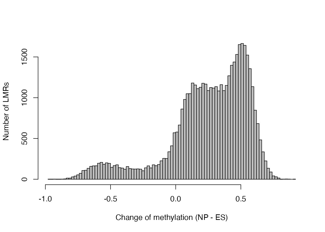
In order to keep the computation time reasonable, we’ll select 10,000 of the LMRs randomly:
Bin genomic regions
Now let’s bin our LMRs by how much they change methylation, using the
bin function from monaLisa.
We are not interested in small changes of methylation, say less than
0.3, so we’ll use the minAbsX argument to create a
no-change bin in [-0.3, 0.3). The remaining LMRs are put into
bins of 800 each:
bins <- bin(x = lmrsel$deltaMeth, binmode = "equalN", nElement = 800,
            minAbsX = 0.3)
table(bins)
#> bins
#> [-0.935,-0.242]  (-0.242,0.327]   (0.327,0.388]   (0.388,0.443]   (0.443,0.491]
#>             800            4400             800             800             800
#>   (0.491,0.536]   (0.536,0.585]   (0.585,0.862]
#>             800             800             800
Generally speaking, we recommend a minimum of ~100 sequences per bin as fewer sequences may lead to small motif counts and thus either small or unstable enrichments.
We can see which bin has been set to be the zero bin using
getZeroBin, or set it to a different bin using
setZeroBin:
# find the index of the level representing the zero bin
levels(bins)
#> [1] "[-0.935,-0.242]" "(-0.242,0.327]"  "(0.327,0.388]"   "(0.388,0.443]"
#> [5] "(0.443,0.491]"   "(0.491,0.536]"   "(0.536,0.585]"   "(0.585,0.862]"
getZeroBin(bins)
#> [1] 2
Because of the asymmetry of methylation changes, there is only a single bin with LMRs that lost methylation and many that gained:
plotBinDensity(lmrsel$deltaMeth, bins)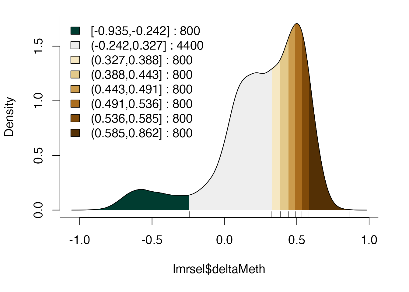
Note that the bin breaks around the no-change bin are not
exactly -0.3 to 0.3. They have been adjusted to have the required 800
LMRs per bin below and above it. monaLisa
will give a warning if the adjusted bin breaks are strongly deviating
from the requested minAbsX value, and
bin(..., model = "breaks") can be used in cases where
exactly defined bin boundaries are required.
Prepare motif enrichment analysis
Next we prepare the motif enrichment analysis. We first need known motifs representing transcription factor binding site preferences. We extract all vertebrate motifs from the JASPAR2020 package as positional weight matrices (PWMs):
pwms <- getMatrixSet(JASPAR2020,
                     opts = list(matrixtype = "PWM",
                                 tax_group = "vertebrates"))
Furthermore, we need the sequences corresponding to our LMRs. As sequences in one bin are compared to the sequences in other bins, we would not want differences of sequence lengths or composition between bins that might bias our motif enrichment results.
In general, we would recommend to use regions of similar or even
equal lengths to avoid a length bias, for example by using a fixed-size
region around the midpoint of each region of interest using
GenomicRanges::resize. In addition, the resized regions may
have to be constrained to the chromosome boundaries using trim:
summary(width(lmrsel))
#>    Min. 1st Qu.  Median    Mean 3rd Qu.    Max.
#>     9.0   213.0   401.0   512.9   676.0  5973.0
lmrsel <- trim(resize(lmrsel, width = median(width(lmrsel)), fix = "center"))
summary(width(lmrsel))
#>    Min. 1st Qu.  Median    Mean 3rd Qu.    Max.
#>     401     401     401     401     401     401
We can now directly extract the corresponding sequences from the BSgenome.Mmusculus.UCSC.mm10 package (assuming you have started the analysis with genomic regions - if you already have sequences, just skip this step)
lmrseqs <- getSeq(BSgenome.Mmusculus.UCSC.mm10, lmrsel)and check for differences in sequence composition between bins using
the plotBinDiagnostics function. “GCfrac” will plot the
distributions of the fraction of G+C bases, and “dinucfreq” creates a
heatmap of average di-nucleotide frequencies in each bin, relative to
the overall average.
plotBinDiagnostics(seqs = lmrseqs, bins = bins, aspect = "GCfrac")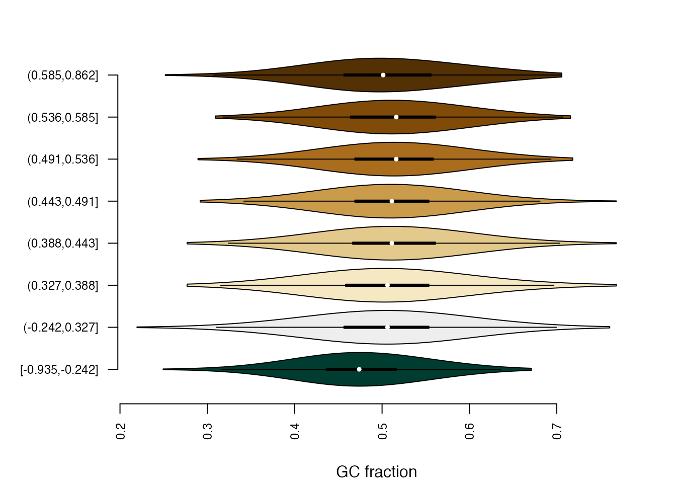
plotBinDiagnostics(seqs = lmrseqs, bins = bins, aspect = "dinucfreq")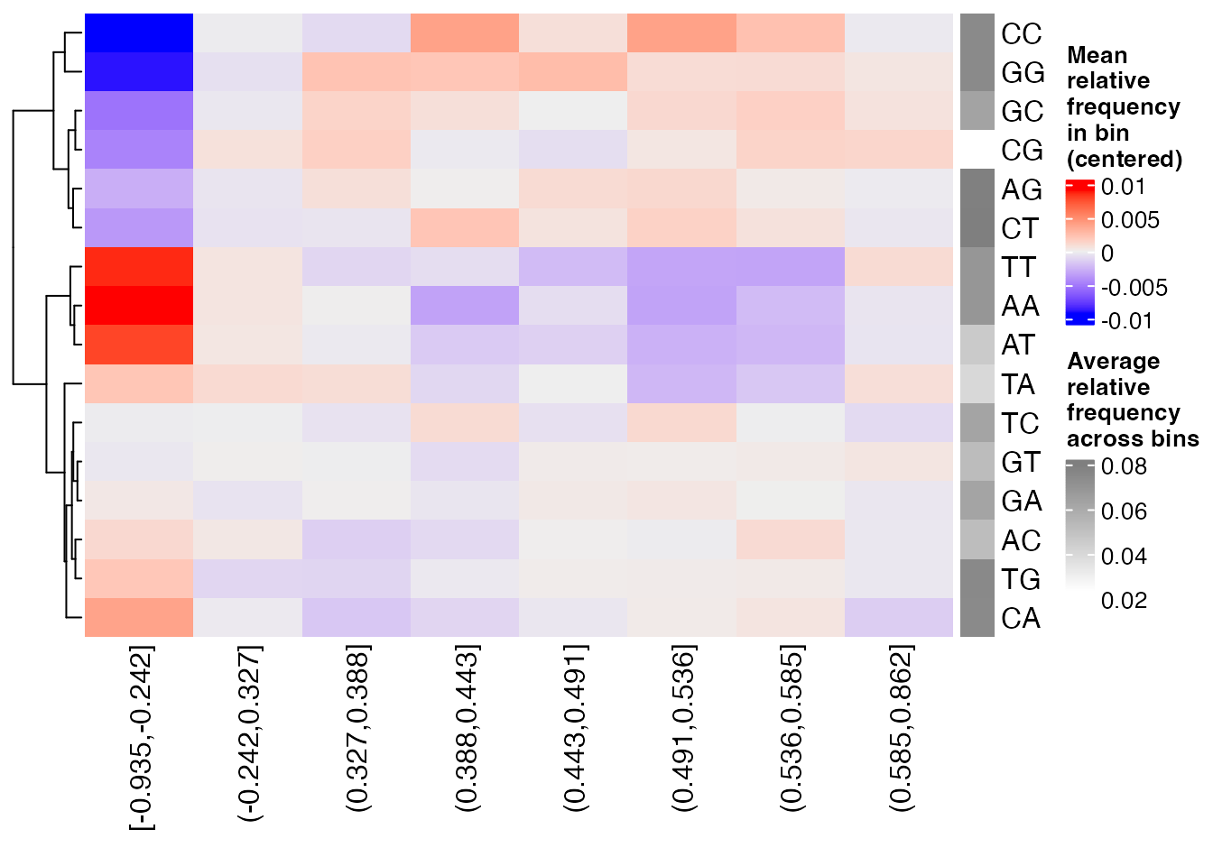
From these plots, we can see that LMRs with lower methylation in NP cells compared to ES cells (bin [-0.935,-0.242]) tend to be GC-poorer than LMRs in other bins. A strong bias of this kind could give rise to false positives in that bin, e.g. enrichments of AT-rich motifs.
At this point in the analysis, it is difficult to decide if this bias
should be addressed here (for example by subsampling sequences of more
comparable GC composition), or if the bias can be ignored because the
built-in sequence composition correction in
calcBinnedMotifEnrR will be able to account for it. Our
recommendation would be to take a mental note at this point and remember
that sequences in the [-0.935,-0.242] bin tend to be GC-poorer. Later,
we should check if AT-rich motifs are specifically enriched in that bin,
and if that is the case, we should critically assess if that result is
robust and can be reproduced in an analysis that uses more balanced
sequences in all bins, or an analysis with
background = "genome". The show_motif_GC and
show_seqlogo arguments of plotMotifHeatmaps
can help to visually identify motif sequence composition in an
enrichment result (see below).
Run motif enrichment analysis
Finally, we run the binned motif enrichment analysis.
This step will take a while, and typically you would use the
BPPARAM argument to run it with parallelization using
n cores as follows:
calcBinnedMotifEnrR(..., BPPARAM = BiocParallel::MulticoreParam(n))).
For this example however, you can skip over the next step and just load
the pre-computed results as shown further below.
se <- calcBinnedMotifEnrR(seqs = lmrseqs, bins = bins, pwmL = pwms)In case you did not run the above code, let’s now read in the results:
se <- readRDS(system.file("extdata", "results.binned_motif_enrichment_LMRs.rds",
                          package = "monaLisa"))
se is a SummarizedExperiment object which
nicely keeps motifs, bins and corresponding metadata together:
# summary
se
#> class: SummarizedExperiment
#> dim: 746 8
#> metadata(5): bins bins.binmode bins.breaks bins.bin0 param
#> assays(7): negLog10P negLog10Padj ... sumForegroundWgtWithHits
#>   sumBackgroundWgtWithHits
#> rownames(746): MA0004.1 MA0006.1 ... MA0528.2 MA0609.2
#> rowData names(5): motif.id motif.name motif.pfm motif.pwm
#>   motif.percentGC
#> colnames(8): [-0.935,-0.242] (-0.242,0.327] ... (0.536,0.585]
#>   (0.585,0.862]
#> colData names(6): bin.names bin.lower ... totalWgtForeground
#>   totalWgtBackground
dim(se) # motifs-by-bins
#> [1] 746   8

# motif info
rowData(se)
#> DataFrame with 746 rows and 5 columns
#>             motif.id   motif.name                       motif.pfm
#>          <character>  <character>                  <PFMatrixList>
#> MA0004.1    MA0004.1         Arnt         MA0004.1; Arnt; Unknown
#> MA0006.1    MA0006.1    Ahr::Arnt    MA0006.1; Ahr::Arnt; Unknown
#> MA0019.1    MA0019.1 Ddit3::Cebpa MA0019.1; Ddit3::Cebpa; Unknown
#> MA0029.1    MA0029.1        Mecom        MA0029.1; Mecom; Unknown
#> MA0030.1    MA0030.1        FOXF2        MA0030.1; FOXF2; Unknown
#> ...              ...          ...                             ...
#> MA0093.3    MA0093.3         USF1         MA0093.3; USF1; Unknown
#> MA0526.3    MA0526.3         USF2         MA0526.3; USF2; Unknown
#> MA0748.2    MA0748.2          YY2          MA0748.2; YY2; Unknown
#> MA0528.2    MA0528.2       ZNF263       MA0528.2; ZNF263; Unknown
#> MA0609.2    MA0609.2         CREM         MA0609.2; CREM; Unknown
#>                                                            motif.pwm
#>                                                       <PWMatrixList>
#> MA0004.1       MA0004.1; Arnt; Basic helix-loop-helix factors (bHLH)
#> MA0006.1  MA0006.1; Ahr::Arnt; Basic helix-loop-helix factors (bHLH)
#> MA0019.1 MA0019.1; Ddit3::Cebpa; Basic leucine zipper factors (bZIP)
#> MA0029.1                   MA0029.1; Mecom; C2H2 zinc finger factors
#> MA0030.1           MA0030.1; FOXF2; Fork head / winged helix factors
#> ...                                                              ...
#> MA0093.3       MA0093.3; USF1; Basic helix-loop-helix factors (bHLH)
#> MA0526.3       MA0526.3; USF2; Basic helix-loop-helix factors (bHLH)
#> MA0748.2                     MA0748.2; YY2; C2H2 zinc finger factors
#> MA0528.2                  MA0528.2; ZNF263; C2H2 zinc finger factors
#> MA0609.2         MA0609.2; CREM; Basic leucine zipper factors (bZIP)
#>          motif.percentGC
#>                <numeric>
#> MA0004.1         64.0893
#> MA0006.1         71.5266
#> MA0019.1         48.3898
#> MA0029.1         28.0907
#> MA0030.1         34.2125
#> ...                  ...
#> MA0093.3         51.0234
#> MA0526.3         51.4931
#> MA0748.2         67.2542
#> MA0528.2         67.4339
#> MA0609.2         53.2402
head(rownames(se))
#> [1] "MA0004.1" "MA0006.1" "MA0019.1" "MA0029.1" "MA0030.1" "MA0031.1"

# bin info
colData(se)
#> DataFrame with 8 rows and 6 columns
#>                       bin.names bin.lower bin.upper bin.nochange
#>                     <character> <numeric> <numeric>    <logical>
#> [-0.935,-0.242] [-0.935,-0.242] -0.935484 -0.242127        FALSE
#> (-0.242,0.327]   (-0.242,0.327] -0.242127  0.327369         TRUE
#> (0.327,0.388]     (0.327,0.388]  0.327369  0.387698        FALSE
#> (0.388,0.443]     (0.388,0.443]  0.387698  0.443079        FALSE
#> (0.443,0.491]     (0.443,0.491]  0.443079  0.490691        FALSE
#> (0.491,0.536]     (0.491,0.536]  0.490691  0.535714        FALSE
#> (0.536,0.585]     (0.536,0.585]  0.535714  0.584707        FALSE
#> (0.585,0.862]     (0.585,0.862]  0.584707  0.862443        FALSE
#>                 totalWgtForeground totalWgtBackground
#>                          <numeric>          <numeric>
#> [-0.935,-0.242]                800            8628.40
#> (-0.242,0.327]                4400            5576.92
#> (0.327,0.388]                  800            9186.26
#> (0.388,0.443]                  800            9186.58
#> (0.443,0.491]                  800            9195.14
#> (0.491,0.536]                  800            9157.61
#> (0.536,0.585]                  800            9163.05
#> (0.585,0.862]                  800            9137.44
head(colnames(se))
#> [1] "[-0.935,-0.242]" "(-0.242,0.327]"  "(0.327,0.388]"   "(0.388,0.443]"
#> [5] "(0.443,0.491]"   "(0.491,0.536]"

# assays: the motif enrichment results
assayNames(se)
#> [1] "negLog10P"                "negLog10Padj"
#> [3] "pearsonResid"             "expForegroundWgtWithHits"
#> [5] "log2enr"                  "sumForegroundWgtWithHits"
#> [7] "sumBackgroundWgtWithHits"
assay(se, "log2enr")[1:5, 1:3]
#>          [-0.935,-0.242] (-0.242,0.327] (0.327,0.388]
#> MA0004.1      -0.4332719    -0.16418567   0.047435758
#> MA0006.1       0.2407477    -0.11995829  -0.005914484
#> MA0019.1      -0.6736372     0.26842621   0.030973190
#> MA0029.1      -0.1475501    -0.12750322   0.088480526
#> MA0030.1      -0.4021844     0.06710565   0.152049687
We can plot the results using the plotMotifHeatmaps
function, e.g. selecting all transcription factor motifs that have a
of at least 4.0 in any bin (corresponding to an
).
FDR values are stored in the negLog10Padj assay:
# select strongly enriched motifs
sel <- apply(assay(se, "negLog10Padj"), 1,
             function(x) max(abs(x), 0, na.rm = TRUE)) > 4.0
sum(sel)
#> [1] 59
seSel <- se[sel, ]

# plot
plotMotifHeatmaps(x = seSel, which.plots = c("log2enr", "negLog10Padj"),
                  width = 2.0, cluster = TRUE, maxEnr = 2, maxSig = 10,
                  show_motif_GC = TRUE)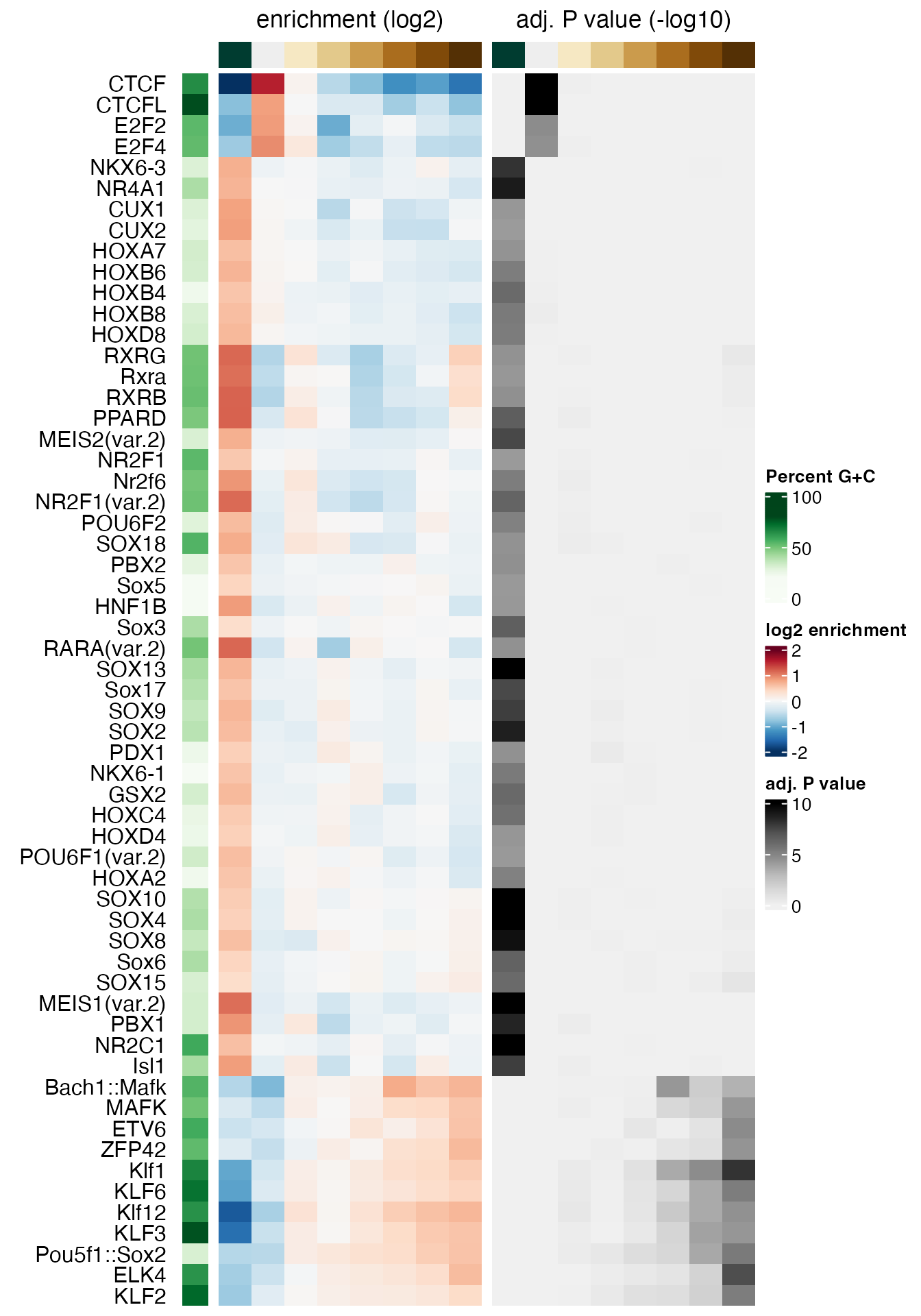
In order to select only motifs with significant enrichments in a specific bin, or in any bin except the “zero” bin, you could use:
# significantly enriched in bin 8
levels(bins)[8]
#> [1] "(0.585,0.862]"
sel.bin8 <- assay(se, "negLog10Padj")[, 8] > 4.0
sum(sel.bin8, na.rm = TRUE)
#> [1] 10

# significantly enriched in any "non-zero" bin
getZeroBin(bins)
#> [1] 2
sel.nonZero <- apply(
    assay(se, "negLog10Padj")[, -getZeroBin(bins), drop = FALSE], 1,
    function(x) max(abs(x), 0, na.rm = TRUE)) > 4.0
sum(sel.nonZero)
#> [1] 55
Setting cluster = TRUE in plotMotifHeatmaps
has re-ordered the rows using hierarchical clustering of the
pearsonResid assay. As many transcription factor binding
motifs are similar to each other, it is also helpful to show the
enrichment heatmap clustered by motif similarity. To this end, we first
calculate all pairwise motif similarities (measured as the maximum
Pearson correlation of all possible shifted alignments). This can be
quickly calculated for the few selected motifs using the
motifSimilarity function. For many motifs, this step may
take a while, and it may be useful to parallelize it using the
BPPARAM argument (e.g. to run on n parallel
threads using the multi-core backend, you can use:
motifSimilarity(..., BPPARAM = BiocParallel::MulticoreParam(n))).
SimMatSel <- motifSimilarity(rowData(seSel)$motif.pfm)
range(SimMatSel)
#> [1] 0.05339967 1.00000000
The order of the TFs in the resulting matrix is consistent with the
elements of seSel, and the maximal similarity between any
pair of motifs is 1.0. By subtracting these similarities from 1.0, we
obtain distances that we use to perform a hierarchical clustering with
the stats::hclust function. The returned object
(hcl) is then passed to the cluster argument
of plotMotifHeatmaps to define the order of the rows in the
heatmap. The plotting of the dendrogram is controlled by the argument
show_dendrogram, and we also display the motifs as sequence
logos using show_seqlogo:
# create hclust object, similarity defined by 1 - Pearson correlation
hcl <- hclust(as.dist(1 - SimMatSel), method = "average")
plotMotifHeatmaps(x = seSel, which.plots = c("log2enr", "negLog10Padj"),
                  width = 1.8, cluster = hcl, maxEnr = 2, maxSig = 10,
                  show_dendrogram = TRUE, show_seqlogo = TRUE,
                  width.seqlogo = 1.2)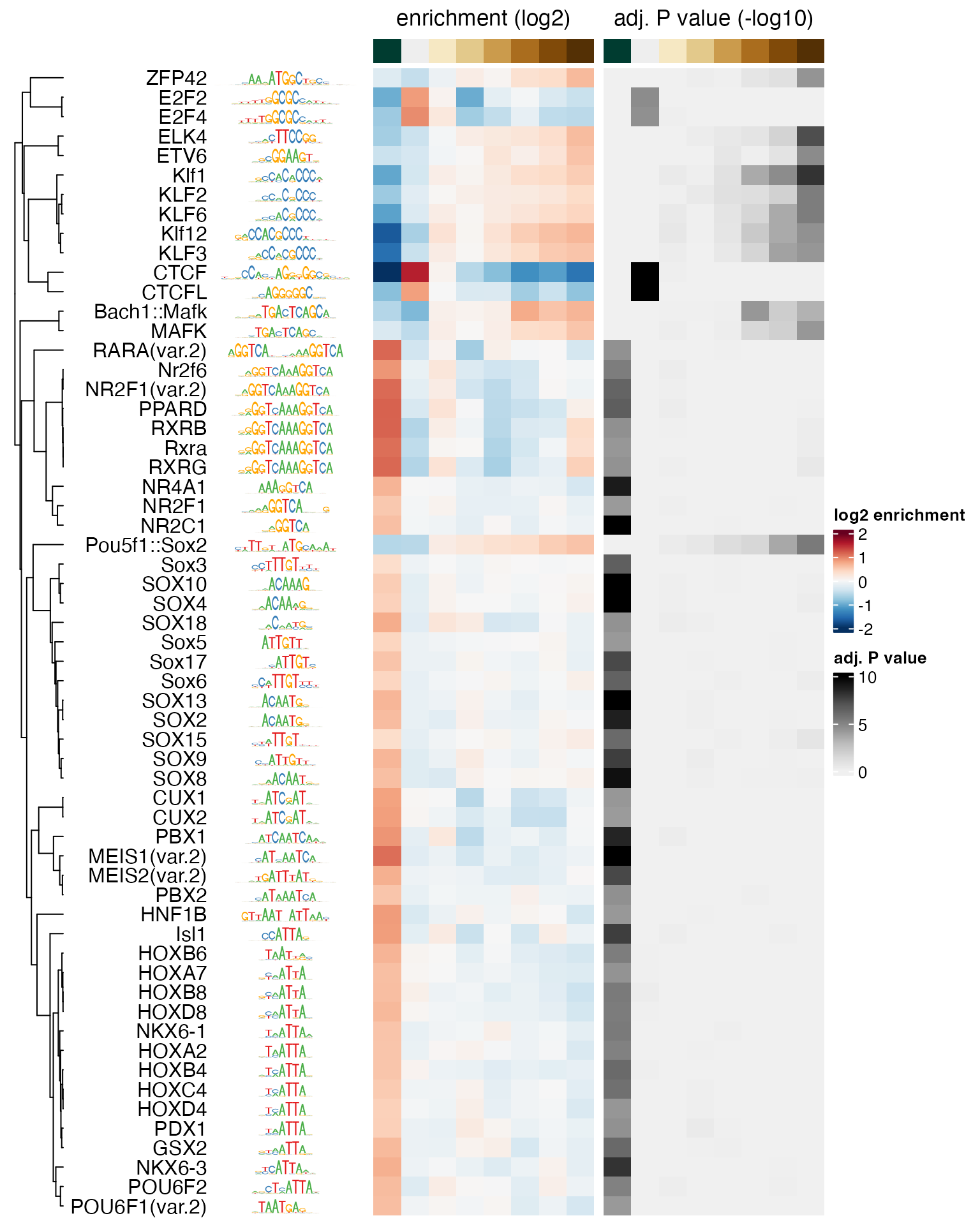
We have seen above that sequences in the [-0.935,-0.242] bin (first
column from the left in the heatmap) were GC-poorer than the sequences
in other bins. While some of the enriched motifs in that bin are not
GC-poor (for example RARA, NR2F1 and similar motifs), other more weakly
enriched motifs are clearly AT-rich (for example HOX family motifs). To
verify that these are not false positive results, the motif analysis
should be repeated after sequences have been subsampled in each bin to
have similar GC composition in all bins, or with
calcBinnedMotifEnrR(..., background = "genome"). The latter
is illustrated in section @ref(vsgenome).
Convert between motif text file for Homer and motif
objects in R
monaLisa
provides two functions for performing binned motif enrichment analysis
(calcBinnedMotifEnrR and
calcBinnedMotifEnrHomer). calcBinnedMotifEnrR
implements the binned motif enrichment analysis in R,
similarly to Homer, and does not require the user to have
the Homer tool pre-installed. For more information on that
function and how it resembles the Homer tool see the
function documentation.
A simple way to represent a DNA sequence motif that assumes
independence of positions in the motif is a matrix with four rows (for
the bases A, C, G and T) and n columns for the
n positions in the motif. The values in that matrix can
represent the sequence preferences of a binding protein in several
different ways:
-
Position frequency matrices (PFM) contain values
that correspond to the number of times (frequency) that a given base has
been observed in at a given position of the motif. It is usually
obtained from a set of known, aligned binding site sequences, and
depending on the number of sequences, the values will be lower or
higher. In
R, PFMs are often represented usingTFBSTools::PFMatrix(single motif) orTFBSTools::PFMatrixList(set of motifs) objects. This is the rawest way to represent a sequence motif and can be converted into any other representation. -
Position probability matrices (PPM) are obtained by
dividing the counts in each column of a PFM by their sum. The values now
give a probability of observing a given base at that position of the
motif and sum up to one in each column. This is the representation used
in motif text files for
Homer. A PPM can only be converted back to a PFM by knowing or assuming how many binding site sequences were observed (see argumentninhomerToPFMatrixList).
-
Position weight matrices (PWM) (also known as
position specific scoring matrices, PSSM) are obtained by comparing the
base probabilities in a PPM to the probabilities of observing each base
outside of a binding site (background base probabilities), for example
by calculating log-odds scores (see
TFBSTools::toPWMfor details). This is a useful representation for scanning sequences for motif matches. InR, PWMs are often represented usingTFBSTools::PWMatrix(single motif) orTFBSTools::PWMatrixList(set of motifs).
calcBinnedMotifEnrR takes PWMs as a
TFBSTools::PWMatrixList object to scan for motif hits.
calcBinnedMotifEnrHomer on the other hand takes a motif
text file with PPMs, and requires the user to have Homer
installed to use it for the binned motif enrichment analysis. Here, we
show how one can get motif PFMs from JASPAR2020
and convert them to a Homer-compatible text file with PPMs
(dumpJaspar) and vice versa
(homerToPFMatrixList), and how to convert a
TFBSTools::PFMatrixList to a
TFBSTools::PWMatrixList for use with
calcBinnedMotifEnrR or findMotifHits:
# get PFMs from JASPAR2020 package (vertebrate subset)
pfms <- getMatrixSet(JASPAR2020,
                     opts = list(matrixtype = "PFM",
                                 tax_group = "vertebrates"))

# convert PFMs to PWMs
pwms <- toPWM(pfms)

# convert JASPAR2020 PFMs (vertebrate subset) to Homer motif file
tmp <- tempfile()
convert <- dumpJaspar(filename = tmp,
                      pkg = "JASPAR2020",
                      pseudocount = 0,
                      opts = list(tax_group = "vertebrates"))

# convert Homer motif file to PFMatrixList
pfms_ret <- homerToPFMatrixList(filename = tmp, n = 100L)

# compare the first PFM
# - notice the different magnitude of counts (controlled by `n`)
# - notice that with the default (recommended) value of `pseudocount = 1.0`,
#   there would be no zero values in pfms_ret matrices, making
#   pfms and pfms_ret even more different
as.matrix(pfms[[1]])
#>   [,1] [,2] [,3] [,4] [,5] [,6]
#> A    4   19    0    0    0    0
#> C   16    0   20    0    0    0
#> G    0    1    0   20    0   20
#> T    0    0    0    0   20    0
as.matrix(pfms_ret[[1]])
#>   [,1] [,2] [,3] [,4] [,5] [,6]
#> A   20   95    0    0    0    0
#> C   80    0  100    0    0    0
#> G    0    5    0  100    0  100
#> T    0    0    0    0  100    0

# compare position probability matrices with the original PFM
round(sweep(x = as.matrix(pfms[[1]]), MARGIN = 2,
            STATS = colSums(as.matrix(pfms[[1]])), FUN = "/"), 3)
#>   [,1] [,2] [,3] [,4] [,5] [,6]
#> A  0.2 0.95    0    0    0    0
#> C  0.8 0.00    1    0    0    0
#> G  0.0 0.05    0    1    0    1
#> T  0.0 0.00    0    0    1    0
round(sweep(x = as.matrix(pfms_ret[[1]]), MARGIN = 2,
            STATS = colSums(as.matrix(pfms_ret[[1]])), FUN = "/"), 3)
#>   [,1] [,2] [,3] [,4] [,5] [,6]
#> A  0.2 0.95    0    0    0    0
#> C  0.8 0.00    1    0    0    0
#> G  0.0 0.05    0    1    0    1
#> T  0.0 0.00    0    0    1    0
Motif enrichment analysis with only one or two sets of sequences
In some cases, we are interested in identifying enriched motifs between just two sets of sequences (binary motif enrichment), for example between ATAC peaks with increased and decreased accessibility. Numerical values that could be used for grouping the regions in multiple bins may not be available. Or we may be interested in analyzing just a single set of sequences (for example a set of ChIP-seq peaks), relative to some neutral background. In this section, we show how such binary or single-set motif enrichment analyses can be performed using monaLisa.
Binary motif enrichment analysis: comparing two sets of sequences
The binary motif enrichment analysis is a simple special case of the general binned motif analysis described in section @ref(binned), where the two sets to be compared are defining the two bins.
Let’s re-use the DNA methylation data from section @ref(binned) and
assume that we just want to compare the sequences that don’t show large
changes in their methylation levels (lmr.unchanged, changes
smaller than 5%) to those that gain more than 60% methylation
(lmr.up):
lmr.unchanged <- lmrsel[abs(lmrsel$deltaMeth) < 0.05]
length(lmr.unchanged)
#> [1] 608

lmr.up <- lmrsel[lmrsel$deltaMeth > 0.6]
length(lmr.up)
#> [1] 630
As before, we need a single sequence object (lmrseqs2,
which is a DNAStringSet) that we obtain by combining these
two groups into a single GRanges object
(lmrsel2) and extract the corresponding sequences from the
genome (lmrseqs2). If you already have two sequence
objects, they can be just concatenated using
lmrseqs2 <- c(seqs.group1, seqs.group2).
# combine the two sets or genomic regions
lmrsel2 <- c(lmr.unchanged, lmr.up)

# extract sequences from the genome
lmrseqs2 <- getSeq(BSgenome.Mmusculus.UCSC.mm10, lmrsel2)
Finally, we manually create a binning factor (bins2)
that defines the group membership for each element in
lmrseqs2:
# define binning vector
bins2 <- rep(c("unchanged", "up"), c(length(lmr.unchanged), length(lmr.up)))
bins2 <- factor(bins2)
table(bins2)
#> bins2
#> unchanged        up
#>       608       630
Now we can run the binned motif enrichment analysis. To keep the
calculation time short, we will just run it on the motifs that we had
selected above in seSel:
se2 <- calcBinnedMotifEnrR(seqs = lmrseqs2, bins = bins2,
                           pwmL = pwms[rownames(seSel)])
se2
#> class: SummarizedExperiment
#> dim: 59 2
#> metadata(5): bins bins.binmode bins.breaks bins.bin0 param
#> assays(7): negLog10P negLog10Padj ... sumForegroundWgtWithHits
#>   sumBackgroundWgtWithHits
#> rownames(59): MA0070.1 MA0077.1 ... MA1113.2 MA0143.4
#> rowData names(5): motif.id motif.name motif.pfm motif.pwm
#>   motif.percentGC
#> colnames(2): unchanged up
#> colData names(6): bin.names bin.lower ... totalWgtForeground
#>   totalWgtBackground
We visualize the results for motifs that are enriched in one of the
two groups with an adjusted p value of less than
(the order of the columns in the heatmap is defined by the order of the
factor levels in bins2, given by levels(bins2)
and can also be obtained from colnames(se2); here it is
unchanged, up):
sel2 <- apply(assay(se2, "negLog10Padj"), 1,
             function(x) max(abs(x), 0, na.rm = TRUE)) > 4.0
sum(sel2)
#> [1] 12

plotMotifHeatmaps(x = se2[sel2,], which.plots = c("log2enr", "negLog10Padj"),
                  width = 1.8, cluster = TRUE, maxEnr = 2, maxSig = 10,
                  show_seqlogo = TRUE)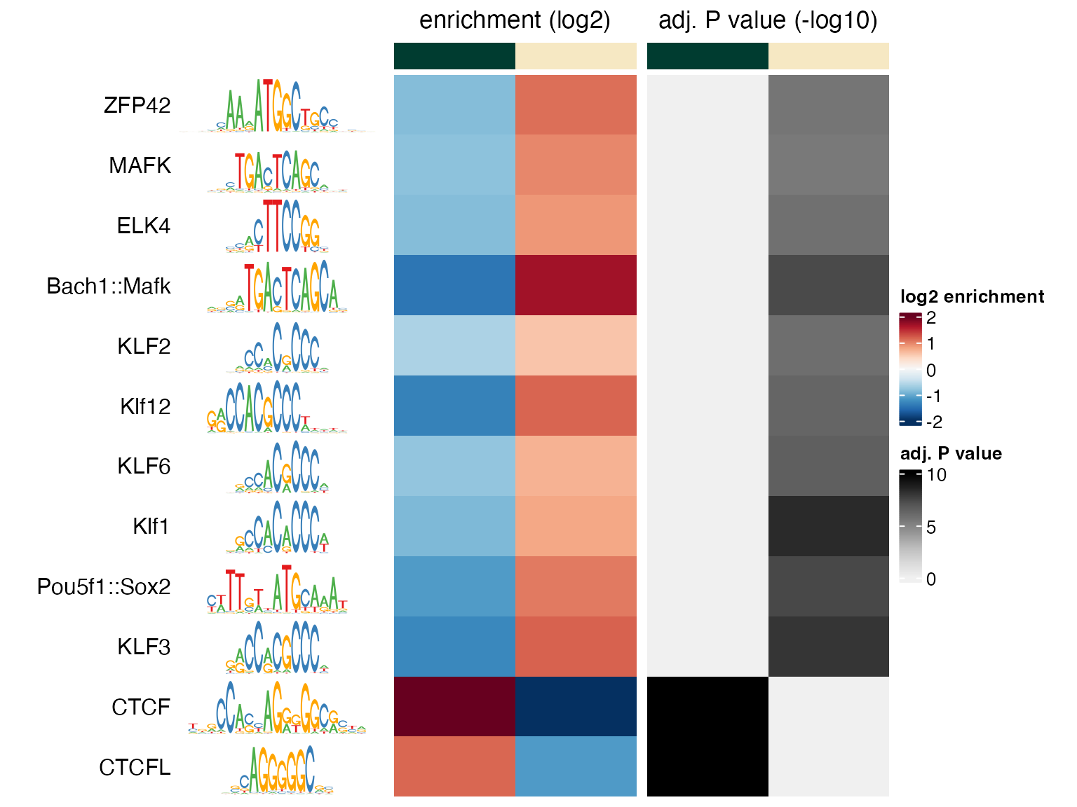
Single set motif enrichment analysis: comparing a set of sequences to a suitable background
Motif enrichments can also be obtained from a single set of genomic regions or sequences (foreground set), by comparing it to a suitable background set. A suitable background set could be for example sequences with a similar sequence composition that are randomly selected from the same genome, or sequences obtained by randomization of the foreground sequences by shuffling or permutation.
A noteworthy package in this context is nullranges that focuses on the selection of such background ranges (representing the null hypothesis), for example controlling for confounding covariates like GC composition. After a suitable background set has been identified using nullranges, a binary motif enrichment analysis as described in section @ref(binary) can be performed. Manually defining the background set is recommended to control for covariates other than GC composition and to get access to the selected background sequences, for example to verify if they are indeed similar to the foreground sequences for those covariates.
A quick alternative with less flexibility in the background set
definition is available directly in monaLisa,
by using calcBinnedMotifEnrR(..., background = "genome").
This will select the background set by randomly sampling sequences from
the genome (given by the genome argument, optionally
restricted to the intervals defined in the genome.regions
argument). For each foreground sequence, genome.oversample
background sequences of the same size (on average) are sampled. From
these, one per foreground sequence is selected trying to best match its
G+C composition.
We apply this simple approach here to check if the motif enrichments identified in section @ref(binned) could be in part false positives due to the GC-poor first bin ([-0.935,-0.242], see above).
Let’s first obtain the sequences from that bin
(lmrseqs3), and then run calcBinnedMotifEnrR
comparing to a genome background. In order to make the sampling
reproducible, we are seeding the random number generator inside the
BPPARAM object. Also, to speed up the calculation, we will
only include the motifs we had selected above in seSel:
lmrseqs3 <- lmrseqs[bins == levels(bins)[1]]
length(lmrseqs3)
#> [1] 800

se3 <- calcBinnedMotifEnrR(seqs = lmrseqs3,
                           pwmL = pwms[rownames(seSel)],
                           background = "genome",
                           genome = BSgenome.Mmusculus.UCSC.mm10,
                           genome.regions = NULL, # sample from full genome
                           genome.oversample = 2,
                           BPPARAM = BiocParallel::SerialParam(RNGseed = 42),
                           verbose = TRUE)
#> ℹ Filtering sequences ...
#> ℹ in total filtering out 0 of 800 sequences (0%)
#> ✔ in total filtering out 0 of 800 sequences (0%) [9ms]
#>
#> ℹ Filtering sequences ...✔ Filtering sequences ... [43ms]
#>
#> ℹ Scanning sequences for motif hits...
#> ✔ Scanning sequences for motif hits... [4.2s]
#>
#> ℹ Create motif hit matrix...
#> ℹ starting analysis of bin 1
#> ✔ starting analysis of bin 1 [6ms]
#>
#> ℹ Create motif hit matrix...ℹ Defining background sequence set (genome)...
#> ✔ Defining background sequence set (genome)... [2.6s]
#>
#> ℹ Create motif hit matrix...ℹ Scanning genomic background sequences for motif hits...
#> ✔ Scanning genomic background sequences for motif hits... [3.7s]
#>
#> ℹ Create motif hit matrix...ℹ Correcting for GC differences to the background sequences...
#> ℹ 8 of 9 GC-bins used (have both fore- and background sequences) 0 of 1600 sequ…
#> ✔ 8 of 9 GC-bins used (have both fore- and background sequences) 0 of 1600 sequ…
#>
#> ℹ Correcting for GC differences to the background sequences...✔ Correcting for GC differences to the background sequences... [66ms]
#>
#> ℹ Create motif hit matrix...ℹ Correcting for k-mer differences between fore- and background sequences...
#> ℹ starting iterative adjustment for k-mer composition (up to 160 iterations)
#> ✔ starting iterative adjustment for k-mer composition (up to 160 iterations) [2…
#>
#> ℹ Correcting for k-mer differences between fore- and background sequences...ℹ 40 of 160 iterations done
#> ✔ 80 of 160 iterations done [169ms]
#>
#> ℹ Correcting for k-mer differences between fore- and background sequences...ℹ 80 of 160 iterations done
#> ✔ 120 of 160 iterations done [169ms]
#>
#> ℹ Correcting for k-mer differences between fore- and background sequences...ℹ 120 of 160 iterations done
#> ✔ 160 of 160 iterations done [170ms]
#>
#> ℹ Correcting for k-mer differences between fore- and background sequences...ℹ 160 of 160 iterations done
#> ℹ     iterations finished
#> ℹ 160 of 160 iterations done✔ 160 of 160 iterations done [18ms]
#>
#> ℹ Correcting for k-mer differences between fore- and background sequences...✔ Correcting for k-mer differences between fore- and background sequences... [7…
#>
#> ℹ Create motif hit matrix...ℹ Calculating motif enrichment...
#> ℹ using Fisher's exact test (one-sided) to calculate log(p-values) for enrichme…
#> ✔ using Fisher's exact test (one-sided) to calculate log(p-values) for enrichme…
#>
#> ℹ Calculating motif enrichment...✔ Calculating motif enrichment... [58ms]
#>
#> ℹ Create motif hit matrix...✔ Create motif hit matrix... [7.3s]
Note that we did not have to provide a bins argument,
and that the result will only have a single column, corresponding to the
single set of sequences that we analyzed:
ncol(se3)
#> [1] 1
When we visualize motifs that are enriched with an adjusted p value
of less than
,
we still find AT-rich motifs significantly enriched, including the HOX
family motifs that were weakly enriched in seSel but for
which it was unclear if their enrichment was driven by the AT-rich
(GC-poor) sequences in that specific bin. The fact that this motif
family is still robustly identified when using a GC-matched genomic
background supports that it may be a real biological signal.
sel3 <- assay(se3, "negLog10Padj")[, 1] > 4.0
sum(sel3)
#> [1] 31

plotMotifHeatmaps(x = se3[sel3,], which.plots = c("log2enr", "negLog10Padj"),
                  width = 1.8, maxEnr = 2, maxSig = 10,
                  show_seqlogo = TRUE)
# analyzed HOX motifs
grep("HOX", rowData(se3)$motif.name, value = TRUE)
#> MA1498.1 MA1499.1 MA1500.1 MA1502.1 MA1504.1 MA1507.1 MA0900.2 MA0910.2
#>  "HOXA7"  "HOXB4"  "HOXB6"  "HOXB8"  "HOXC4"  "HOXD4"  "HOXA2"  "HOXD8"

# significant HOX motifs
grep("HOX", rowData(se3)$motif.name[sel3], value = TRUE)
#> MA1498.1 MA1499.1 MA1500.1 MA1502.1 MA1504.1 MA1507.1 MA0900.2 MA0910.2
#>  "HOXA7"  "HOXB4"  "HOXB6"  "HOXB8"  "HOXC4"  "HOXD4"  "HOXA2"  "HOXD8"
A comparison of log2 motif enrichments between the
background = "otherBins" and
background = "genome" analyses also supports this
conclusion: The HOX family motifs (shown in red) are similarly enriched
in both analyses, while the depletion of GC-rich KLF family motifs
(shown in green) is less pronounced in
background = "genome" and thus more sensitive to the used
background. The depletion of KLF family motifs may thus be an example of
an incorrect result, although note that the depletion was not
significant in either of the two analyses:
cols <- rep("gray", nrow(se3))
cols[grep("HOX", rowData(se3)$motif.name)] <- "#DF536B"
cols[grep("KLF|Klf", rowData(se3)$motif.name)] <- "#61D04F"
par(mar = c(5, 5, 2, 2) + .1, mgp = c(1.75, 0.5, 0), cex = 1.25)
plot(assay(seSel, "log2enr")[,1], assay(se3, "log2enr")[,1],
     col = cols, pch = 20, asp = 1,
     xlab = "Versus other bins (log2 enr)",
     ylab = "Versus genome (log2 enr)")
legend("topleft", c("HOX family","KLF family","other"), pch = 20, bty = "n",
       col = c("#DF536B", "#61D04F", "gray"))
abline(a = 0, b = 1)
abline(h = 0, lty = 3)
abline(v = 0, lty = 3)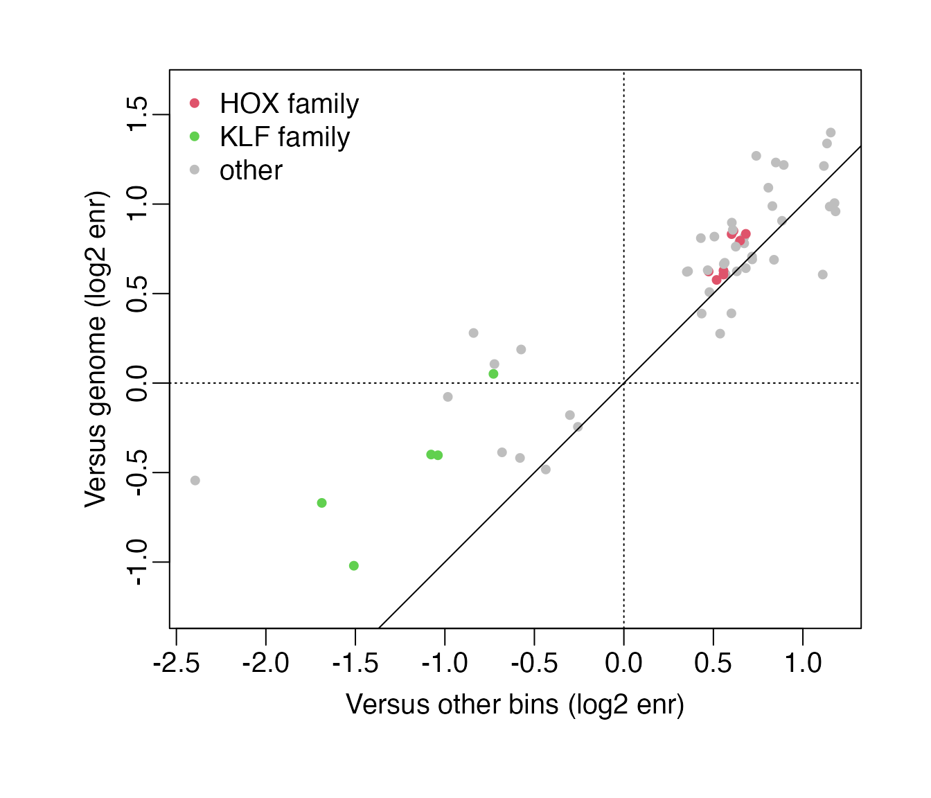
Binned k-mer enrichment analysis
In some situations it may be beneficial to perform the enrichment analysis in a more ‘unbiased’ way, using k-mers rather than annotated motifs. Here, we will illustrate the process using the same LMR data set as used for the motif enrichment analysis above in section @ref(binned). Similarly to the motif enrichment, this step takes a while to perform, and we can also skip over the next step and load the processed object directly.
sekm <- calcBinnedKmerEnr(seqs = lmrseqs, bins = bins, kmerLen = 6,
                          includeRevComp = TRUE)
sekm <- readRDS(system.file(
    "extdata", "results.binned_6mer_enrichment_LMRs.rds",
    package = "monaLisa"
))
Just as for the motif enrichment analysis, the return value is a
SummarizedExperiment object, with the same set of assays
and annotations.
sekm
#> class: SummarizedExperiment
#> dim: 4096 8
#> metadata(5): bins bins.binmode bins.breaks bins.bin0 param
#> assays(7): negLog10P negLog10Padj ... sumForegroundWgtWithHits
#>   sumBackgroundWgtWithHits
#> rownames(4096): AAAAAA AAAAAC ... TTTTTG TTTTTT
#> rowData names(5): motif.id motif.name motif.pfm motif.pwm
#>   motif.percentGC
#> colnames(8): [-0.935,-0.242] (-0.242,0.327] ... (0.536,0.585]
#>   (0.585,0.862]
#> colData names(6): bin.names bin.lower ... totalWgtForeground
#>   totalWgtBackground
As for the motif enrichment, we can extract any k-mer that is enriched in any of the bins.
selkm <- apply(assay(sekm, "negLog10Padj"), 1,
               function(x) max(abs(x), 0, na.rm = TRUE)) > 4
sum(selkm)
#> [1] 85
sekmSel <- sekm[selkm, ]
Next, let’s compare the enriched k-mers to the motifs that were found
earlier. This can be done using the motifKmerSimilarity
function. By showing the similarity between the enriched k-mers and
motifs, we can see whether, e.g., strongly enriched k-mers do not seem
to correspond to an annotated motif.
pfmSel <- rowData(seSel)$motif.pfm
sims <- motifKmerSimilarity(x = pfmSel,
                            kmers = rownames(sekmSel),
                            includeRevComp = TRUE)
dim(sims)
#> [1] 59 85

maxwidth <- max(sapply(TFBSTools::Matrix(pfmSel), ncol))
seqlogoGrobs <- lapply(pfmSel, seqLogoGrob, xmax = maxwidth)
hmSeqlogo <- rowAnnotation(logo = annoSeqlogo(seqlogoGrobs, which = "row"),
                           annotation_width = unit(1.5, "inch"),
                           show_annotation_name = FALSE
)
Heatmap(sims,
        show_row_names = TRUE, row_names_gp = gpar(fontsize = 8),
        show_column_names = TRUE, column_names_gp = gpar(fontsize = 8),
        name = "Similarity", column_title = "Selected TFs and enriched k-mers",
        col = colorRamp2(c(0, 1), c("white", "red")),
        right_annotation = hmSeqlogo)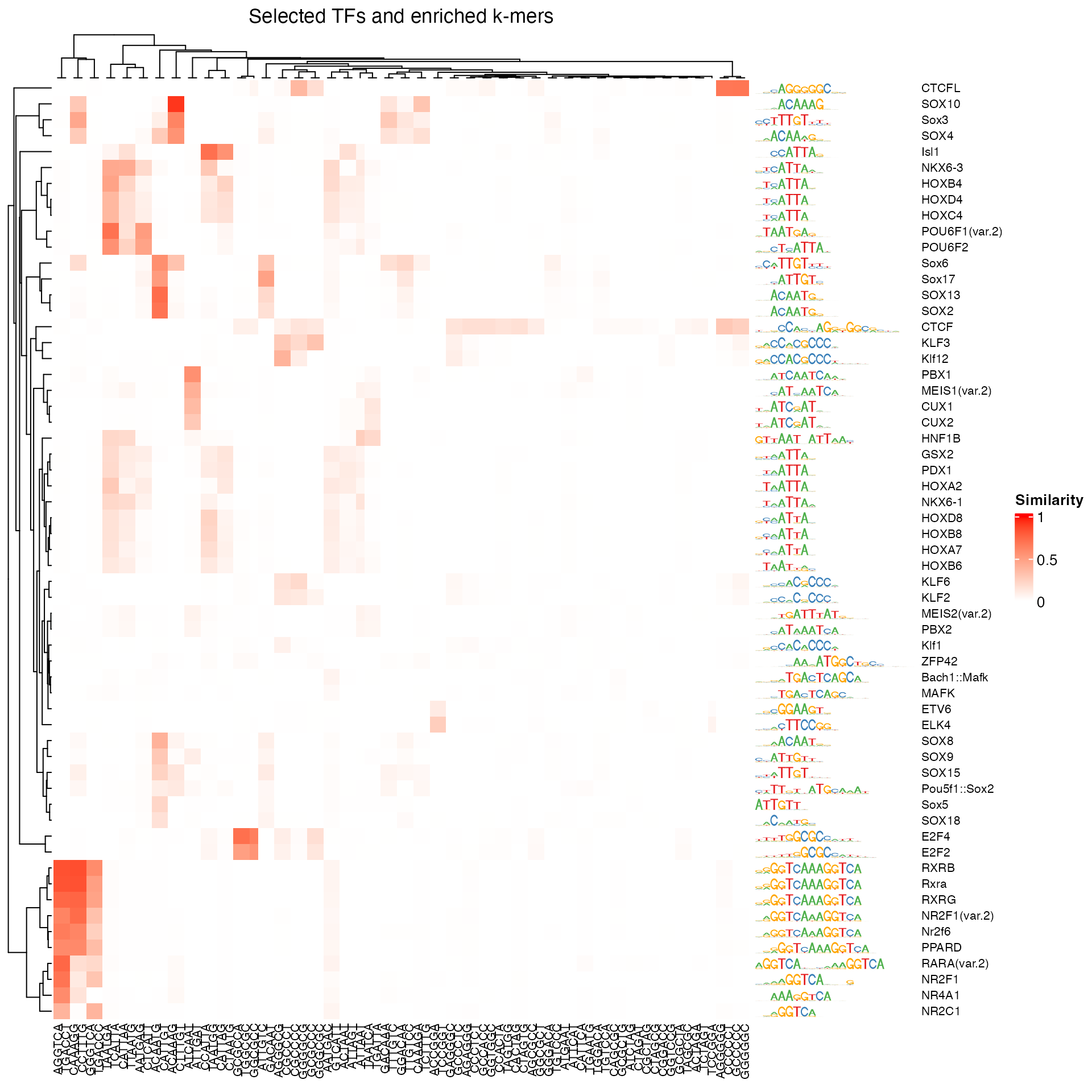
Use monaLisa to annotate genomic regions with predicted motifs
As mentioned, monaLisa can also be used to scan sequences for motifs. For a quick description of motif representations see section @ref(motifConvert). Here is an example (just on a few sequences/motifs for illustration):
# get sequences of promoters as a DNAStringSet
# (the `subject` of `findMotifHits` could also be a single DNAString,
#  or the name of a fasta file)
library(TxDb.Mmusculus.UCSC.mm10.knownGene)
#> Loading required package: GenomicFeatures
#> Loading required package: AnnotationDbi
gr <- trim(promoters(TxDb.Mmusculus.UCSC.mm10.knownGene,
                     upstream = 1000, downstream = 500)[c(1, 4, 5, 10)])
library(BSgenome.Mmusculus.UCSC.mm10)
seqs <- getSeq(BSgenome.Mmusculus.UCSC.mm10, gr)
seqs
#> DNAStringSet object of length 4:
#>     width seq                                               names
#> [1]  1500 CCCTTTTGGATAGATTCTAGGCT...GCTGATTTATGAGTAAGGGATGT ENSMUST00000193812.1
#> [2]  1500 TGCGGTATGTTCATGTATACATG...ATGAATTTACCAATGCCACACAG ENSMUST00000161581.1
#> [3]  1500 TGATTAAGAAAATTCCCTGGTGG...CCCTTGGTGTGGTAGTCACGTCC ENSMUST00000192183.1
#> [4]  1500 TGGAAATGTCTTCCCTCACCCCT...AGGAACCTAGCCTGTCACCCGCA ENSMUST00000195361.1

# get motifs as a PWMatrixList
# (the `query` of `findMotifHits` could also be a single PWMatrix,
#  or the name of a motif file)
library(JASPAR2020)
library(TFBSTools)
pfms <- getMatrixByID(JASPAR2020, c("MA0885.1", "MA0099.3", "MA0033.2",
                                    "MA0037.3", "MA0158.1"))
pwms <- toPWM(pfms)
pwms
#> PWMatrixList of length 5
#> names(5): MA0885.1 MA0099.3 MA0033.2 MA0037.3 MA0158.1
name(pwms)
#>   MA0885.1   MA0099.3   MA0033.2   MA0037.3   MA0158.1
#>     "Dlx2" "FOS::JUN"    "FOXL1"    "GATA3"    "HOXA5"

# predict hits in sequences
res <- findMotifHits(query = pwms,
                     subject = seqs,
                     min.score = 6.0,
                     method = "matchPWM",
                     BPPARAM = BiocParallel::SerialParam())
res
#> GRanges object with 115 ranges and 4 metadata columns:
#>                     seqnames    ranges strand |     matchedSeq    pwmid pwmname
#>                        <Rle> <IRanges>  <Rle> | <DNAStringSet>    <Rle>   <Rle>
#>     [1] ENSMUST00000193812.1    93-100      + |       CTCTTATG MA0158.1   HOXA5
#>     [2] ENSMUST00000193812.1   103-110      + |       AGCTAATT MA0158.1   HOXA5
#>     [3] ENSMUST00000193812.1   252-259      + |       GTCATTAT MA0885.1    Dlx2
#>     [4] ENSMUST00000193812.1   355-362      + |       TGATAAAT MA0037.3   GATA3
#>     [5] ENSMUST00000193812.1   358-365      + |       TAAATTAT MA0885.1    Dlx2
#>     ...                  ...       ...    ... .            ...      ...     ...
#>   [111] ENSMUST00000195361.1   742-749      - |       ATGAAATT MA0158.1   HOXA5
#>   [112] ENSMUST00000195361.1   833-840      - |       ACAATTAT MA0885.1    Dlx2
#>   [113] ENSMUST00000195361.1   842-849      - |       GTAATTAA MA0885.1    Dlx2
#>   [114] ENSMUST00000195361.1   844-851      - |       AAGTAATT MA0158.1   HOXA5
#>   [115] ENSMUST00000195361.1   865-872      - |       ACCATTAT MA0885.1    Dlx2
#>             score
#>         <numeric>
#>     [1]   6.98342
#>     [2]   7.96626
#>     [3]   6.64334
#>     [4]   6.76273
#>     [5]   6.36851
#>     ...       ...
#>   [111]   6.61929
#>   [112]  10.61685
#>   [113]  10.97719
#>   [114]   7.96626
#>   [115]   6.28806
#>   -------
#>   seqinfo: 4 sequences from an unspecified genome

# create hit matrix:
# number of sites of each motif per sequence
m <- table(factor(seqnames(res), levels = names(seqs)),
           factor(res$pwmname, levels = name(pwms)))
m
#>
#>                        Dlx2 FOS::JUN FOXL1 GATA3 HOXA5
#>   ENSMUST00000193812.1    4        2    12     7    10
#>   ENSMUST00000161581.1   10        1     3     5    10
#>   ENSMUST00000192183.1    4        2     2     3    13
#>   ENSMUST00000195361.1   11        1     5     0    10
The transformation of sequence and PWM names to factors with defined
levels in the creation of the hit matrix above is not strictly needed,
but it ensures that even sequences or motifs without any hits are
reported in the matrix, and that the order of sequences (rows) and
motifs (columns) is identical to the order in seqs and
pwms.
Session info and logo
The monaLisa logo uses a drawing that was obtained from http://vectorish.com/lisa-simpson.html under the Creative Commons attribution - non-commercial 3.0 license: https://creativecommons.org/licenses/by-nc/3.0/.
This vignette was built using:
sessionInfo()
#> R Under development (unstable) (2026-01-26 r89334)
#> Platform: aarch64-apple-darwin20
#> Running under: macOS Sequoia 15.7.3
#>
#> Matrix products: default
#> BLAS:   /System/Library/Frameworks/Accelerate.framework/Versions/A/Frameworks/vecLib.framework/Versions/A/libBLAS.dylib
#> LAPACK: /Library/Frameworks/R.framework/Versions/4.6-arm64/Resources/lib/libRlapack.dylib;  LAPACK version 3.12.1
#>
#> locale:
#> [1] en_US.UTF-8/en_US.UTF-8/en_US.UTF-8/C/en_US.UTF-8/en_US.UTF-8
#>
#> time zone: UTC
#> tzcode source: internal
#>
#> attached base packages:
#> [1] grid      stats4    stats     graphics  grDevices utils     datasets
#> [8] methods   base
#>
#> other attached packages:
#>  [1] TxDb.Mmusculus.UCSC.mm10.knownGene_3.10.0
#>  [2] GenomicFeatures_1.63.1
#>  [3] AnnotationDbi_1.73.0
#>  [4] circlize_0.4.17
#>  [5] ComplexHeatmap_2.27.0
#>  [6] monaLisa_1.17.1
#>  [7] BSgenome.Mmusculus.UCSC.mm10_1.4.3
#>  [8] BSgenome_1.79.1
#>  [9] rtracklayer_1.71.3
#> [10] BiocIO_1.21.0
#> [11] Biostrings_2.79.4
#> [12] XVector_0.51.0
#> [13] TFBSTools_1.49.0
#> [14] JASPAR2020_0.99.10
#> [15] SummarizedExperiment_1.41.0
#> [16] Biobase_2.71.0
#> [17] MatrixGenerics_1.23.0
#> [18] matrixStats_1.5.0
#> [19] GenomicRanges_1.63.1
#> [20] Seqinfo_1.1.0
#> [21] IRanges_2.45.0
#> [22] S4Vectors_0.49.0
#> [23] BiocGenerics_0.57.0
#> [24] generics_0.1.4
#> [25] BiocStyle_2.39.0
#>
#> loaded via a namespace (and not attached):
#>  [1] DBI_1.2.3                   bitops_1.0-9
#>  [3] stabs_0.6-4                 rlang_1.1.7
#>  [5] magrittr_2.0.4              clue_0.3-66
#>  [7] GetoptLong_1.1.0            compiler_4.6.0
#>  [9] RSQLite_2.4.5               png_0.1-8
#> [11] systemfonts_1.3.1           vctrs_0.7.1
#> [13] pwalign_1.7.0               pkgconfig_2.0.3
#> [15] shape_1.4.6.1               crayon_1.5.3
#> [17] fastmap_1.2.0               labeling_0.4.3
#> [19] caTools_1.18.3              Rsamtools_2.27.0
#> [21] rmarkdown_2.30              ragg_1.5.0
#> [23] DirichletMultinomial_1.53.0 purrr_1.2.1
#> [25] bit_4.6.0                   xfun_0.56
#> [27] glmnet_4.1-10               cachem_1.1.0
#> [29] cigarillo_1.1.0             jsonlite_2.0.0
#> [31] blob_1.3.0                  DelayedArray_0.37.0
#> [33] BiocParallel_1.45.0         parallel_4.6.0
#> [35] cluster_2.1.8.1             R6_2.6.1
#> [37] bslib_0.10.0                RColorBrewer_1.1-3
#> [39] jquerylib_0.1.4             Rcpp_1.1.1
#> [41] bookdown_0.46               iterators_1.0.14
#> [43] knitr_1.51                  splines_4.6.0
#> [45] Matrix_1.7-4                tidyselect_1.2.1
#> [47] abind_1.4-8                 yaml_2.3.12
#> [49] doParallel_1.0.17           codetools_0.2-20
#> [51] curl_7.0.0                  lattice_0.22-7
#> [53] tibble_3.3.1                KEGGREST_1.51.1
#> [55] withr_3.0.2                 S7_0.2.1
#> [57] evaluate_1.0.5              survival_3.8-6
#> [59] desc_1.4.3                  pillar_1.11.1
#> [61] BiocManager_1.30.27         foreach_1.5.2
#> [63] RCurl_1.98-1.17             ggplot2_4.0.1
#> [65] scales_1.4.0                gtools_3.9.5
#> [67] glue_1.8.0                  seqLogo_1.77.0
#> [69] tools_4.6.0                 TFMPvalue_1.0.0
#> [71] GenomicAlignments_1.47.0    fs_1.6.6
#> [73] XML_3.99-0.20               tidyr_1.3.2
#> [75] colorspace_2.1-2            restfulr_0.0.16
#> [77] cli_3.6.5                   textshaping_1.0.4
#> [79] S4Arrays_1.11.1             dplyr_1.1.4
#> [81] gtable_0.3.6                sass_0.4.10
#> [83] digest_0.6.39               SparseArray_1.11.10
#> [85] rjson_0.2.23                farver_2.1.2
#> [87] memoise_2.0.1               htmltools_0.5.9
#> [89] pkgdown_2.2.0.9000          lifecycle_1.0.5
#> [91] httr_1.4.7                  GlobalOptions_0.1.3
#> [93] bit64_4.6.0-1