This chapter describes how to read footprinting data from modBam files and other formats into R. It also introduces how the data is represented in memory. SingleMoleculeGenomicsIO provides four functions for reading data into R from specific file types: readModBam, readMismatchBam, readBedMethyl and readModkitExtract. If you want to jump right in, have a look at the documentation of the reader function corresponding to the type of your data.
We start by loading the required packages and a BSgenome object providing the mouse genome sequence.
Typically, single molecule footprinting data at the single read level is stored in modBam files, which are standard bam files (Li et al. (2009)) that in addition to the usual information on alignments also contain base modifications encoded in the ML and MM tags (see section 1.7 of SAMtags.pdf for details).
readModBam reads modBam files and can either keep the data at the level of individual reads or summarize them per genomic position and sample. This is controlled via the level argument to readModBam. By default, read-level data is imported. In fact, SingleMoleculeGenomicsIO provides two modes for importing read-level data: level = "quickread" is often the fastest, but does not return the full set of read-level annotations, and is not compatible with read sampling. level = "read" on the other hand provides a more complete output, but is a bit slower. If level is not specified, SingleMoleculeGenomicsIO will select the best mode based on the other arguments provided to readModBam (specifically, whether variant names or read sampling are requested). As illustrated in Section 2.4 below, summary data (aggregated across reads) can also be imported by setting level = "summary".
2.2 Data representation
Let’s start by reading individual reads from a modBam file for a small region of the genome:
Show/hide code
se <-readModBam(bamfiles =c(wt1 ="data/mESC_wt_6mA_rep1.bam",wt2 ="data/mESC_wt_6mA_rep2.bam"),modbase ="a", regions ="chr8:39286000-39286200", seqinfo =seqinfo(gnm), sequenceContextWidth =1, sequenceReference = gnm,trim =TRUE)se
Here is a scheme that illustrates the internals of se containing read-level data:
Figure 2.1
Let’s go through the individual parts. You can see that the data is contained in a RangedSummarizedExperiment object. This is a container that contains one or more assays (here only one assay called mod_prob). Each assay is a matrix-like object and contains the loaded data (here: base modification probabilities of individual reads).
Show/hide code
assayNames(se)
[1] "mod_prob"
The rows represent genomic positions and the columns represent samples. In our example, we have loaded data from two modBam files corresponding to the two samples "wt1" and "wt2", thus the object has two columns:
Show/hide code
ncol(se)
[1] 2
Show/hide code
colnames(se)
[1] "wt1" "wt2"
The 209 rows correspond to individual base positions, for which at least one modification has been loaded. You can get the genomic coordinates of these positions using rowRanges:
Show/hide code
nrow(se)
[1] 209
Show/hide code
rowRanges(se)
UnstitchedGPos object with 209 positions and 1 metadata column:
        seqnames       pos strand | sequenceContext
           <Rle> <integer>  <Rle> |  <DNAStringSet>
    [1]     chr8  39286000      - |               G
    [2]     chr8  39286001      - |               A
    [3]     chr8  39286002      + |               A
    [4]     chr8  39286003      - |               A
    [5]     chr8  39286004      + |               A
    ...      ...       ...    ... .             ...
  [205]     chr8  39286196      + |               A
  [206]     chr8  39286197      - |               A
  [207]     chr8  39286198      + |               A
  [208]     chr8  39286199      + |               A
  [209]     chr8  39286200      - |               C
  -------
  seqinfo: 61 sequences (1 circular) from mm39 genome
These positions are stranded, as base modifications can be observed on either of the two strands:
Show/hide code
table(strand(se))
  +   -   *
105 104   0
Finally, the individual reads of a sample are stored in the assay, inside the “column” of that sample:
You can see that each column is itself an object of type NaMatrix.
Show/hide code
# get the NaMatrix with reads of sample wt1mp1 <-assay(se, "mod_prob")$wt1mp1
<209 x 47 NaMatrix> of type "double" [nnacount=3179 (32%)]:
       wt1-039b9bb6-f9e0-4ac0-937d-09f69f6030d3 ... wt1-f77f5ae9-dd3a-4e08-a390-7e80868433a7
  [1,]                                       NA   .                                       NA
  [2,]                                        0   .                                        0
  [3,]                                       NA   .                                       NA
  [4,]                                        0   .                                        0
  [5,]                                       NA   .                                       NA
   ...                                        .   .                                        .
[205,]                                       NA   .                                       NA
[206,]                                        0   .                                0.1503906
[207,]                                       NA   .                                       NA
[208,]                                       NA   .                                       NA
[209,]                                       NA   .                                       NA
The rows in the NaMatrix corresponding to the same genomic positions we have seen above, but the columns correspond to the 47 individual reads. The numeric values correspond to modification probabilities. For Oxford Nanopore data, a value greater than 0.5 or 0.7 is typically considered modified. Many values are NA (missing), either because a read did not overlap a given position, or there was no information about modifications at that position in that read. Storing all these NA values would be a waste of memory, which is avoided in the NaMatrix, which is a special type of sparse matrix from the SparseArray package that only stores non-NA values.
Here is an illustration of the summary-level data container:
Figure 2.2
Its dimensions are identical to the original se (positions by samples), however it contains additional assays that do not have the nested structure with individual reads, but are simple matrices:
By default, flattenReadLevelAssay keeps the read-level assay ("mod_prob") and generates summarized assays with the numbers of modified and total bases ("Nmod" and "Nvalid"), and the fraction of modified bases per position and sample ("FracMod").
2.4 Directly reading summary-level data
If the individual reads are not required, you can directly summarize them while reading, which is faster and eliminates the call to flattenReadLevelAssay. This is achieved by adding the argument level = "summary" to the readModBam call:
In some cases, we may want to read a random set of reads from a modBam file, for example to calculate average modification rates or quality statistics. In such cases, reading data by genomic position is not optimal.
readModBam provides a special reading mode for this, controlled by the arguments nAlnsToSample and seqnamesToSampleFrom:
For details of how to make the sampling reproducible even when using multiple parallel threads, and why you might get a lower number of sampled reads than requested, please look at the documentation of readModBam.
2.6 Improving reading performance
Even though readModBam is implemented using C/C++ for speed and efficiency, reading the data may become slow. Here are a few points that may help to reduce the time to read modification data from modBam files:
Read summary-level data: Reading of summary-level data (argument level = "summary") is much faster than reading of read-level data, so use it whenever you do not need to represent indidvual reads.
Parallelization: readModBam supports parallel processing, controlled by the BPPARAM argument. If multiple workers are available in the BPPARAM object (see BiocParallel), they will be used to read data from from multiple modBam files in parallel. If the number of workers is larger than the number of bamfiles, the workers will further be used to speed-up decompression of bam records.
Region size: If you are reading read-level data from large or many regions, certain operations like sub-setting of positions may become slow. It may overall be faster to call readModBam multiple times on fewer or smaller regions, and keeping track of the partial results, than calling readModBam a single time on all regions.
2.7 Reading from other file types
In addition to reading from modBam files, you can also read data from mismatchBam files, e.g. resulting from Bisulfite-seq or deaminase-based experiments aligned with QuasR or bismark, using readMismatchBam, summary-level data from bedMethyl files using readBedMethyl, or from tabular files created by modkit using readModkitExtract. The arguments of these reader functions are largely similar to the ones used for reading modBam files.
Li, Heng, Bob Handsaker, Alec Wysoker, Tim Fennell, Jue Ruan, Nils Homer, Gabor Marth, Goncalo Abecasis, Richard Durbin, and 1000 Genome Project Data Processing Subgroup. 2009. “The Sequence Alignment/Map Format and SAMtools.”Bioinformatics 25 (16): 2078–79.
Source Code
# Reading data from files {#sec-reading-data}This chapter describes how to read footprinting data from `modBam` files and other formats into R.It also introduces how the data is represented in memory.[fmicompbio/SingleMoleculeGenomicsIO]{.githubpkg} provides four functions for reading data into R from specific file types: [readModBam]{.fnio}, [readMismatchBam]{.fnio}, [readBedMethyl]{.fnio} and [readModkitExtract]{.fnio}.If you want to jump right in, have a look at the documentation of the reader function corresponding to the type of your data.We start by loading the required packages and a `BSgenome` object providing the mouse genome sequence.```{r}#| message: false#| label: load-packagesBSgenomeName <-"BSgenome.Mmusculus.GENCODE.GRCm39.gencodeM34"library(SingleMoleculeGenomicsIO)library(BiocParallel)library(BSgenomeName, character.only =TRUE)library(SummarizedExperiment)library(SparseArray)# Load genomegnm <-get(BSgenomeName)genome(gnm) <-"mm39"```## Read-level versus summary-levelTypically, single molecule footprinting data at the single read level is stored in `modBam` files, which are standard `bam` files (@Li2009-kl) that in addition to the usual information on alignments also contain base modifications encoded in the `ML` and `MM` tags (see section 1.7 of [SAMtags.pdf](https://samtools.github.io/hts-specs/SAMtags.pdf) for details).[readModBam]{.fnio} reads `modBam` files and can either keep the data at the level of individual reads or summarize them per genomic position and sample.This is controlled via the `level` argument to [readModBam]{.fnio}.By default, read-level data is imported.In fact, [fmicompbio/SingleMoleculeGenomicsIO]{.githubpkg} provides two modes for importing read-level data: `level = "quickread"` is often the fastest, but does not return the full set of read-level annotations, and is not compatible with read sampling.`level = "read"` on the other hand provides a more complete output, but is a bit slower. If `level` is not specified, [fmicompbio/SingleMoleculeGenomicsIO]{.githubpkg} will select the best mode based on the other arguments provided to [readModBam]{.fnio} (specifically, whether variant names or read sampling are requested).As illustrated in @sec-summary-data below, summary data (aggregated across reads) can also be imported by setting `level = "summary"`.## Data representation {#sec-data-representation}Let's start by reading individual reads from a `modBam` file for a small region of the genome:```{r}#| label: read-modbam-readlevelse <-readModBam(bamfiles =c(wt1 ="data/mESC_wt_6mA_rep1.bam",wt2 ="data/mESC_wt_6mA_rep2.bam"),modbase ="a", regions ="chr8:39286000-39286200", seqinfo =seqinfo(gnm), sequenceContextWidth =1, sequenceReference = gnm,trim =TRUE)se```Here is a scheme that illustrates the internals of `se` containing read-level data: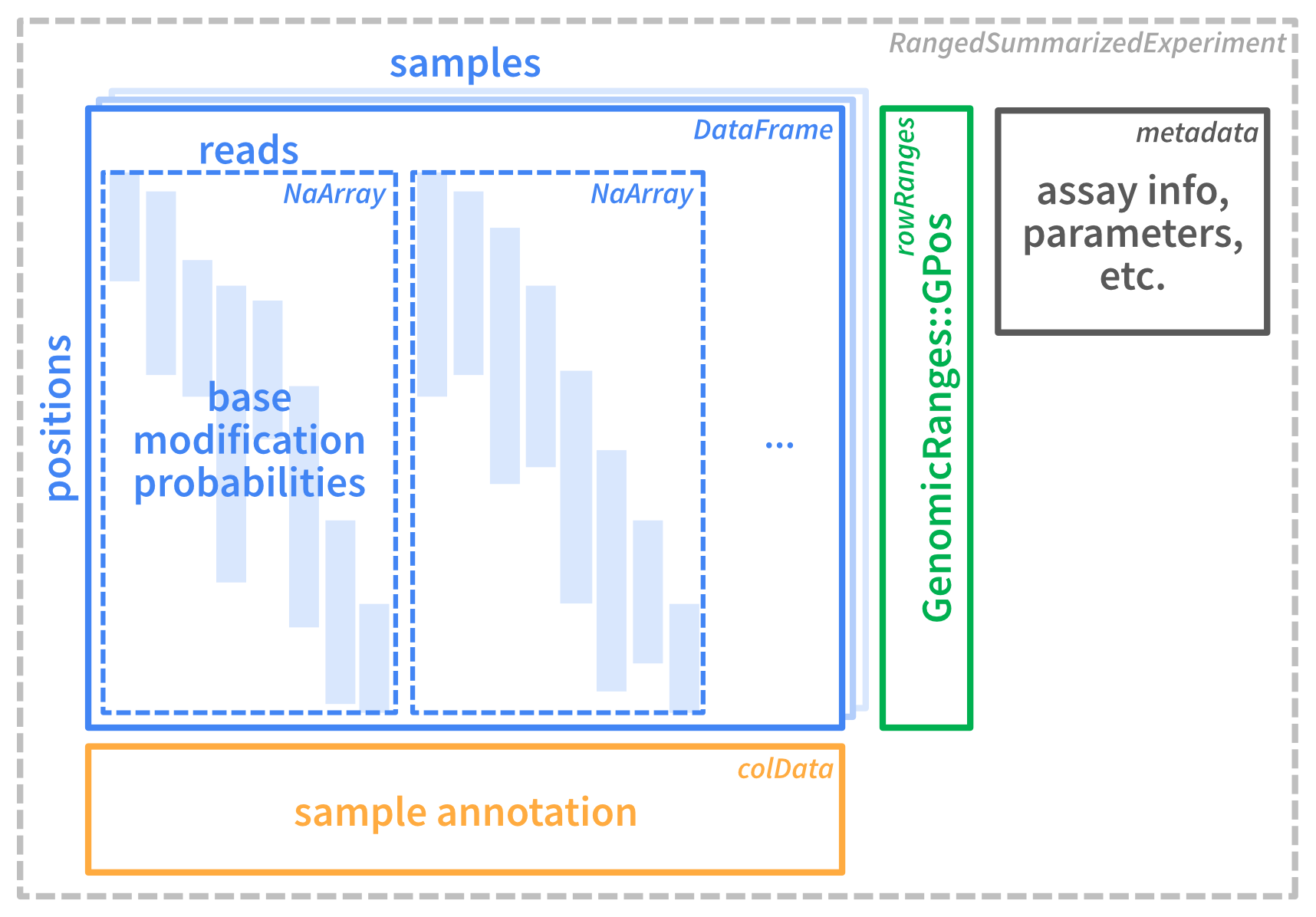{#fig-schematic-readlevel .lightbox fig-alt="SummarizedExperiment with read-level data in assays." height=300}Let's go through the individual parts.You can see that the data is contained in a `RangedSummarizedExperiment` object.This is a container that contains one or more assays (here only one assay called `mod_prob`). Each assay is a matrix-like object and contains the loaded data (here: base modification probabilities of individual reads).```{r}#| label: show-assaynamesassayNames(se)```The rows represent genomic positions and the columns represent samples.In our example, we have loaded data from two `modBam` files corresponding to the two samples `"wt1"` and `"wt2"`, thus the object has two columns:```{r}#| label: show-colnamesncol(se)colnames(se)```The `r nrow(se)` rows correspond to individual base positions, for which at least one modification has been loaded. You can get the genomic coordinates of these positions using `rowRanges`:```{r}#| label: show-rowrangesnrow(se)rowRanges(se)```These positions are stranded, as base modifications can be observed on either of the two strands:```{r}#| label: show-strandtable(strand(se))```Finally, the individual reads of a sample are stored in the assay, inside the "column" of that sample:```{r}#| label: show-modprobassayNames(se)assay(se, "mod_prob")```You can see that each column is itself an object of type `NaMatrix`.```{r}#| label: show-namatrix# get the NaMatrix with reads of sample wt1mp1 <-assay(se, "mod_prob")$wt1mp1```The rows in the `NaMatrix` corresponding to the same genomic positions we have seen above, but the columns correspond to the `r ncol(mp1)` individual reads.The numeric values correspond to modification probabilities.For Oxford Nanopore data, a value greater than 0.5 or 0.7 is typically considered modified.Many values are `NA` (missing), either because a read did not overlap a given position, or there was no information about modifications at that position in that read.Storing all these `NA` values would be a waste of memory, which is avoided in the `NaMatrix`, which is a special type of sparse matrix from the [SparseArray]{.biocpkg} package that only stores non-`NA` values.## Flattening read-level to summary-level dataWe can use [flattenReadLevelAssay]{.fnio} to go from this read-level to summary-level data:```{r}#| label: flatten-sese_summary <-flattenReadLevelAssay(se)```Here is an illustration of the summary-level data container: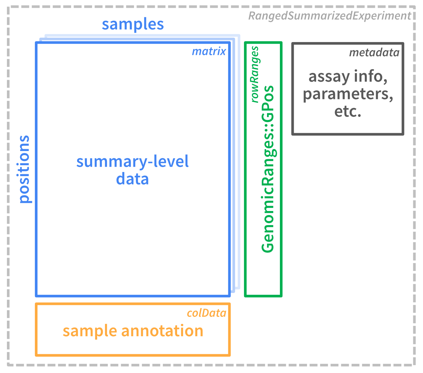{#fig-schematic-summarylevel .lightbox fig-alt="SummarizedExperiment with summary-level data in assays." height=300}Its dimensions are identical to the original `se` (positions by samples), however it contains additional assays that do not have the nested structure with individual reads, but are simple matrices:```{r}#| label: show-summary-assaysdim(se_summary)assayNames(se_summary)head(assay(se_summary, "Nmod"))```By default, [flattenReadLevelAssay]{.fnio} keeps the read-level assay (`"mod_prob"`) and generates summarized assays with the numbers of modified and total bases (`"Nmod"` and `"Nvalid"`), and the fraction of modified bases per position and sample (`"FracMod"`).## Directly reading summary-level data {#sec-summary-data}If the individual reads are not required, you can directly summarize them while reading, which is faster and eliminates the call to [flattenReadLevelAssay]{.fnio}.This is achieved by adding the argument `level = "summary"` to the [readModBam]{.fnio} call:```{r}#| label: read-modbam-summarylevelse_summary_direct <-readModBam(bamfiles =c(wt1 ="data/mESC_wt_6mA_rep1.bam",wt2 ="data/mESC_wt_6mA_rep2.bam"),modbase ="a", regions ="chr8:39286000-39286200", seqinfo =seqinfo(gnm), sequenceContextWidth =1, sequenceReference = gnm,trim =TRUE,level ="summary")se_summary_directidentical(assay(se_summary, "FracMod"),assay(se_summary_direct, "FracMod"))```## Read sampling {#sec-read-sampling}In some cases, we may want to read a random set of reads from a `modBam` file, for example to calculate average modification rates or quality statistics.In such cases, reading data by genomic position is not optimal.[readModBam]{.fnio} provides a special reading mode for this, controlled by the arguments `nAlnsToSample` and `seqnamesToSampleFrom`:```{r}#| label: read-modbam-samplese_sampled <-readModBam(bamfiles =c(wt1 ="data/mESC_wt_6mA_rep1.bam",wt2 ="data/mESC_wt_6mA_rep2.bam"),modbase ="a", seqinfo =seqinfo(gnm), sequenceContextWidth =1, sequenceReference = gnm,nAlnsToSample =20,seqnamesToSampleFrom ="chr19")se_sampledse_sampled$n_reads```For details of how to make the sampling reproducible even when using multiple parallel threads, and why you might get a lower number of sampled reads than requested, please look at the documentation of [readModBam]{.fnio}.## Improving reading performanceEven though [readModBam]{.fnio} is implemented using C/C++ for speed and efficiency, reading the data may become slow.Here are a few points that may help to reduce the time to read modification data from `modBam` files:- *Read summary-level data*: Reading of summary-level data (argument `level = "summary"`) is much faster than reading of read-level data, so use it whenever you do not need to represent indidvual reads. - *Parallelization*: [readModBam]{.fnio} supports parallel processing, controlled by the `BPPARAM` argument. If multiple workers are available in the `BPPARAM` object (see [BiocParallel]{.biocpkg}), they will be used to read data from from multiple `modBam` files in parallel. If the number of workers is larger than the number of `bamfiles`, the workers will further be used to speed-up decompression of bam records.- *Region size*: If you are reading read-level data from large or many `regions`, certain operations like sub-setting of positions may become slow. It may overall be faster to call [readModBam]{.fnio} multiple times on fewer or smaller `regions`, and keeping track of the partial results, than calling [readModBam]{.fnio} a single time on all `regions`.## Reading from other file typesIn addition to reading from `modBam` files, you can also read data from `mismatchBam` files, e.g. resulting from Bisulfite-seq or deaminase-based experiments aligned with [QuasR]{.biocpkg} or `bismark`, using [readMismatchBam]{.fnio}, summary-level data from `bedMethyl` files using [readBedMethyl]{.fnio}, or from tabular files created by `modkit` using [readModkitExtract]{.fnio}.The arguments of these reader functions are largely similar to the ones used for reading `modBam` files.```{r}#| label: read-other-formats# read from mismatchBam### TODO# read from bedMethylbmfile <-system.file("extdata", "modkit_pileup_5mC_1.bed.gz",package ="SingleMoleculeGenomicsIO")se_bedmethyl <-readBedMethyl(fnames = bmfile,modbase ="m",seqinfo =seqinfo(gnm), sequenceContextWidth =3, sequenceReference = gnm)se_bedmethyl# read from a tabular file created by modkitextrfile <-system.file("extdata", "modkit_extract_rc_5mC_1.tsv.gz",package ="SingleMoleculeGenomicsIO")se_modkit <-readModkitExtract(fnames = extrfile,modbase ="m",filter =NULL,seqinfo =seqinfo(gnm), sequenceContextWidth =3, sequenceReference = gnm)se_modkit```## Session info<details><summary><b>Click to view session info</b></summary>```{r}#| label: session-infosessioninfo::session_info(info ="packages")```</details>

