Run Exon-Intron Split Analysis.

Starting from count tables with exonic and intronic counts for two conditions, perform all the steps in EISA (normalize, identify quantifyable genes, calculate contrasts and their significance).

runEISA(
  cntEx,
  cntIn,
  cond,
  method = NULL,
  modelSamples = TRUE,
  geneSelection = c("filterByExpr", "none", "Gaidatzis2015"),
  statFramework = c("QLF", "LRT"),
  legacyQLF = FALSE,
  effects = c("predFC", "Gaidatzis2015"),
  pscnt = 2,
  sizeFactor = c("exon", "intron", "individual"),
  recalcNormFactAfterFilt = TRUE,
  recalcLibSizeAfterFilt = FALSE,
  ...
)

Arguments

cntEx

Gene by sample matrix with exonic counts, OR a SummarizedExperiment with two assays named exon and intron, containing exonic and intronic counts, respectively. If cntEx is a SummarizedExperiment, cntIn will be disregarded.

cntIn

Gene by sample matrix with intronic counts. Must have the same structure as cntEx (same number and order of rows and columns) if cntEx is a matrix. Will be disregarded if cntEx is a SummarizedExperiment.

cond

numeric, character or factor with two levels that groups the samples (columns of cntEx and cntIn) into two conditions. The contrast will be defined as secondLevel - firstLevel.

method

One of NULL (the default) or "Gaidatzis2015". If "Gaidatzis2015", gene filtering, statistical analysis and calculation of contrasts is performed as described in Gaidatzis et al. 2015, and the statistical analysis is based on glmFit and glmLRT. This is done by setting the arguments modelSamples, geneSelection, effects, pscnt, statFramework, sizeFactor, recalcNormFactAfterFilt and recalcLibSizeAfterFilt to appropriate values (see details), overriding the defaults or any value passed to these arguments. If NULL, the default values of the arguments will be used instead (recommended).

modelSamples

Whether to include a sample identifier in the design matrix of the statistical model. If TRUE, potential sample effects that affect both exonic and intronic counts of that sample will be taken into account, which could result in higher sensitivity (default: TRUE).

geneSelection

Controls how to select quantifyable genes. One of the following:

"filterByExpr":: (default) First, counts are normalized using calcNormFactors, treating intronic and exonic counts as individual samples. Then, filterByExpr is used with default parameters to select quantifyable genes.
"none":: This will use all the genes provided in the count tables, assuming that an appropriate selection of quantifyable genes has already been done.
"Gaidatzis2015":: First, intronic and exonic counts are linearly scaled to the mean library size (estimated as the sum of all intronic or exonic counts, respectively). Then, quantifyable genes are selected as the genes with counts x that fulfill log2(x + 8) > 5 in both exons and introns.

statFramework

Selects the framework within edgeR that is used for the statistical analysis. One of:

"QLF":: (default) Quasi-likelihood F-test using glmQLFit and glmQLFTest. This framework is highly recommended as it gives stricter error rate control by accounting for the uncertainty in dispersion estimation.
"LRT":: Likelihood ratio test using glmFit and glmLRT

legacyQLF

Whether to use the 'legacy' version of glmQLFit. See glmQLFit for more details. If FALSE, the new method introduced in edgeR 4.0.0 is used.

effects

How the effects (contrasts or log2 fold-changes) are calculated. One of:

"predFC":: (default) Fold-changes are calculated using the fitted model with predFC with prior.count = pscnt. Please note that if a sample factor is included in the model (modelSamples=TRUE), effects cannot be obtained from that model. In that case, effects are obtained from a simpler model without sample effects.
"Gaidatzis2015":: Fold-changes are calculated using the formula log2((x + pscnt)/(y + pscnt)). If pscnt is not set to 8, runEISA will warn that this deviates from the method used in Gaidatzis et al., 2015.

pscnt

numeric(1) with pseudocount to add to read counts (default: 2). For method = "Gaidatzis2015", it is set to 8. It is added to scaled read counts used in geneSelection = "Gaidatzis2015" and effects = "Gaidatzis2015", or else used in cpm(..., prior.count = pscnt) and predFC(..., prior.count = pscnt).

sizeFactor

How the size factors are calculated in the analysis. If 'exon' (default), the exon-derived size factors are used also for the columns corresponding to intronic counts. If 'intron', the intron-derived size factors are used also for the columns corresponding to exonic counts. If 'individual', column-wise size factors are calculated.

recalcNormFactAfterFilt

Logical, indicating whether normalization factors should be recalculated after filtering out lowly expressed genes.

recalcLibSizeAfterFilt

Logical, indicating whether library sizes should be recalculated after filtering out lowly expressed genes.

...

additional arguments passed to the DGEList constructor, such as lib.size or genes.

Value

a list with elements

fracIn: fraction intronic counts in each sample
contrastName: contrast name
contrasts: contrast matrix for quantifyable genes, with average log2 fold-changes in exons (Dex), in introns (Din), and average difference between log2 fold-changes in exons and introns (Dex.Din)
DGEList: DGEList object used in model fitting
tab.ExIn: statisical results for differential changes between exonic and intronic contrast, an indication for post-transcriptional regulation.
contr.ExIn: contrast vector used for testing the difference between exonic and intronic contrast (results in tab.ExIn)
designMatrix: design matrix used for testing the difference between exonic and intronic contrast (results in tab.ExIn)
params: a list with parameter values used to run EISA

Details

Setting method = "Gaidatzis2015" has precedence over other argument values and corresponds to setting: modelSamples = FALSE, geneSelection = "Gaidatzis2015", statFramework = "LRT", effects = "Gaidatzis2015", pscnt = 8, sizeFactor = "individual", recalcNormFactAfterFilt = TRUE, recalcLibSizeAfterFilt = FALSE.

References

Analysis of intronic and exonic reads in RNA-seq data characterizes transcriptional and post-transcriptional regulation. Dimos Gaidatzis, Lukas Burger, Maria Florescu and Michael B. Stadler Nature Biotechnology, 2015 Jul;33(7):722-9. doi: 10.1038/nbt.3269.

Author

Michael Stadler

Examples

cntEx <- readRDS(system.file("extdata", "Fig3abc_GSE33252_rawcounts_exonic.rds",
                             package = "eisaR"))[,-1]
cntIn <- readRDS(system.file("extdata", "Fig3abc_GSE33252_rawcounts_intronic.rds",
                             package = "eisaR"))[,-1]
cond <- factor(c("ES","ES","TN","TN"))
res <- runEISA(cntEx, cntIn, cond)
#> filtering quantifyable genes...
#> keeping 11759 from 20288 (58%)
#> fitting statistical model...
#> done
#> calculating log-fold changes...
#> done
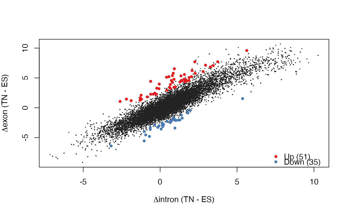
plotEISA(res)
#> identified 139 genes to highlight