Using ez-zarr in R

This vignette describes how to use the ezzarr R package, which provides a thin R wrapper around the ez-zarr python package. For a full documentation of the functionality provided by ez-zarr, we refer to the website.

ezzarr does not add any new functionality compared to the python package, but provides an easy way to set up and activate a conda environment with all necessary dependencies for ez-zarr, and once the environment is activated in an R session, the reticulate package can be used to access the functionality in ez-zarr, to import and interact with image and plate objects from OME-Zarr files in R.

Load the `ezzarr` package

library(ezzarr)
library(EBImage)

Check the version of ez-zarr

The getEzZarrVersion() function returns the version of ez-zarr which will be installed and used by the current version of ezzarr. Calling this function will also build the conda environment if it does not already exist.

getEzZarrVersion()
#> [1] "0.3.8"

Get the path to the environment

ezzarr provides a convenience function to get the path to the ez-zarr conda environment. This can be useful e.g. in order to activate the environment outside of R.

getEzZarrEnvPath()
#> [1] "/Users/runner/Library/Caches/org.R-project.R/R/basilisk/1.21.0/ezzarr/0.1.5/ezzarr"

Download example data to temporary directory

In the remainder of this vignette, we will illustrate the use of ezzarr by means of an example data set, representing a maximum intensity projection of one well from a high-content screening plate, processed using Fractal. The same data set is used in the ez-zarr python documentation. The data is available on Zenodo; here, we download and unpack it to a temporary directory.

td <- tempdir()
url <- "https://zenodo.org/records/10519143/files/20200812-CardiomyocyteDifferentiation14-Cycle1_mip.zarr.zip"
download.file(url, destfile = file.path(td, basename(url)))
unzip(file.path(td, basename(url)), 
      exdir = td)

Before going further, we save the path to the unpacked data set in the zarrpath variable, and explore the content of the directory.

zarrpath <- file.path(td, sub("\\.zip$", "", basename(url)))
fs::dir_tree(zarrpath, recurse = 3)
#> /var/folders/w5/_8wgjw3j5cg6mgrth3s2kg9m0000gn/T//Rtmp9J2Urn/20200812-CardiomyocyteDifferentiation14-Cycle1_mip.zarr
#> └── B
#>     └── 03
#>         └── 0
#>             ├── 0
#>             ├── 1
#>             ├── 2
#>             ├── 3
#>             ├── 4
#>             ├── labels
#>             └── tables

Activate the environment

Next, we activate the conda environment that contains ez-zarr and all necessary dependencies, via the enableEzZarr() function. In addition to activating the conda environment, this function returns a list of imported python modules, which can be used to access python functions.

## Activate environment
env <- enableEzZarr()

## List imported modules
names(env)
#> [1] "plt"     "np"      "ez_zarr"

## Switch matplotlib backend (for non-interactive use)
env$plt$switch_backend("agg")

Load an example image

Now that the environment is activated, we can import an image from an OME-Zarr fileset. We do this by creating an object of the Image class, defined in ez-zarr.

img <- env$ez_zarr$ome_zarr$Image(path = file.path(zarrpath, "B/03/0"))

img
#> Image 0
#>   path: /var/folders/w5/_8wgjw3j5cg6mgrth3s2kg9m0000gn/T//Rtmp9J2Urn/20200812-CardiomyocyteDifferentiation14-Cycle1_mip.zarr/B/03/0
#>   n_channels: 1 (DAPI)
#>   n_pyramid_levels: 5
#>   pyramid_zyx_scalefactor: [1. 2. 2.]
#>   full_resolution_zyx_spacing (micrometer): [1.0, 0.1625, 0.1625]
#>   segmentations: empty, nuclei
#>   tables (measurements): FOV_ROI_table, expected_table_FOV_ROI_table_1_False_0_0, expected_table_FOV_ROI_table_1_True_0_0, expected_table_masked_nuclei_ROI_table_0_True_0_0, expected_table_masked_nuclei_ROI_table_1_True_0_0, expected_table_well_ROI_table_0_True_0_0, expected_table_well_ROI_table_3_False_0_0, expected_table_well_ROI_table_3_True_0_0, nuclei, nuclei_ROI_table, well_ROI_table

img$tree(level = 1)
#> /
#>  ├── 0 (1, 1, 2160, 5120) uint16
#>  ├── 1 (1, 1, 1080, 2560) uint16
#>  ├── 2 (1, 1, 540, 1280) uint16
#>  ├── 3 (1, 1, 270, 640) uint16
#>  ├── 4 (1, 1, 135, 320) uint16
#>  ├── labels
#>  └── tables

Get details about the image

ez-zarr contains many methods for accessing various aspects of an Image object. Here, we illustrate some of these.

## Channel information
length(img$nchannels_image)
#> [1] 1
img$channels[[1]]
#> $color
#> [1] "00FFFF"
#> 
#> $label
#> [1] "DAPI"
#> 
#> $wavelength_id
#> [1] "A01_C01"
#> 
#> $window
#> $window$end
#> [1] 800
#> 
#> $window$max
#> [1] 65535
#> 
#> $window$min
#> [1] 0
#> 
#> $window$start
#> [1] 110

## Label names
img$label_names
#> [1] "empty"  "nuclei"

## Scales for a given pyramid level
unlist(img$get_scale(pyramid_level = "2"))
#> [1] 1.00 1.00 0.65 0.65

## Path
img$get_path()
#> [1] "/var/folders/w5/_8wgjw3j5cg6mgrth3s2kg9m0000gn/T//Rtmp9J2Urn/20200812-CardiomyocyteDifferentiation14-Cycle1_mip.zarr/B/03/0"

## Image name
img$name
#> [1] "0"

## Table names
img$table_names
#>  [1] "FOV_ROI_table"                                    
#>  [2] "expected_table_FOV_ROI_table_1_False_0_0"         
#>  [3] "expected_table_FOV_ROI_table_1_True_0_0"          
#>  [4] "expected_table_masked_nuclei_ROI_table_0_True_0_0"
#>  [5] "expected_table_masked_nuclei_ROI_table_1_True_0_0"
#>  [6] "expected_table_well_ROI_table_0_True_0_0"         
#>  [7] "expected_table_well_ROI_table_3_False_0_0"        
#>  [8] "expected_table_well_ROI_table_3_True_0_0"         
#>  [9] "nuclei"                                           
#> [10] "nuclei_ROI_table"                                 
#> [11] "well_ROI_table"

Plot image

Plots in ez-zarr are implemented using matplotlib.pyplot and display correctly when using the plot methods interactively from python (e.g. img.plot()) or from R via reticulate (e.g. img$plot()). A special case is the use of plot methods in non-interactive Rmarkdown or Quarto documents. In these, the plots are only shown for python code chunks, which is used in the examples below (note the r.img syntax to refer to the img object in the R process).

With default settings

r.img.plot()

The corresponding R code (for interactive use) would look like:

img$plot()

Adding a scale bar, limiting the channel range

r.img.plot(channels = [0],
           channel_colors = ["white"],
           channel_ranges = [[100, 600]],
           scalebar_micrometer = 150,
           scalebar_color = "yellow",
           scalebar_position = "topleft",
           scalebar_label = True,
           fig_width_inch = 5,
           fig_height_inch = 4,
           fig_dpi = 100,
           axis_style = "micrometer")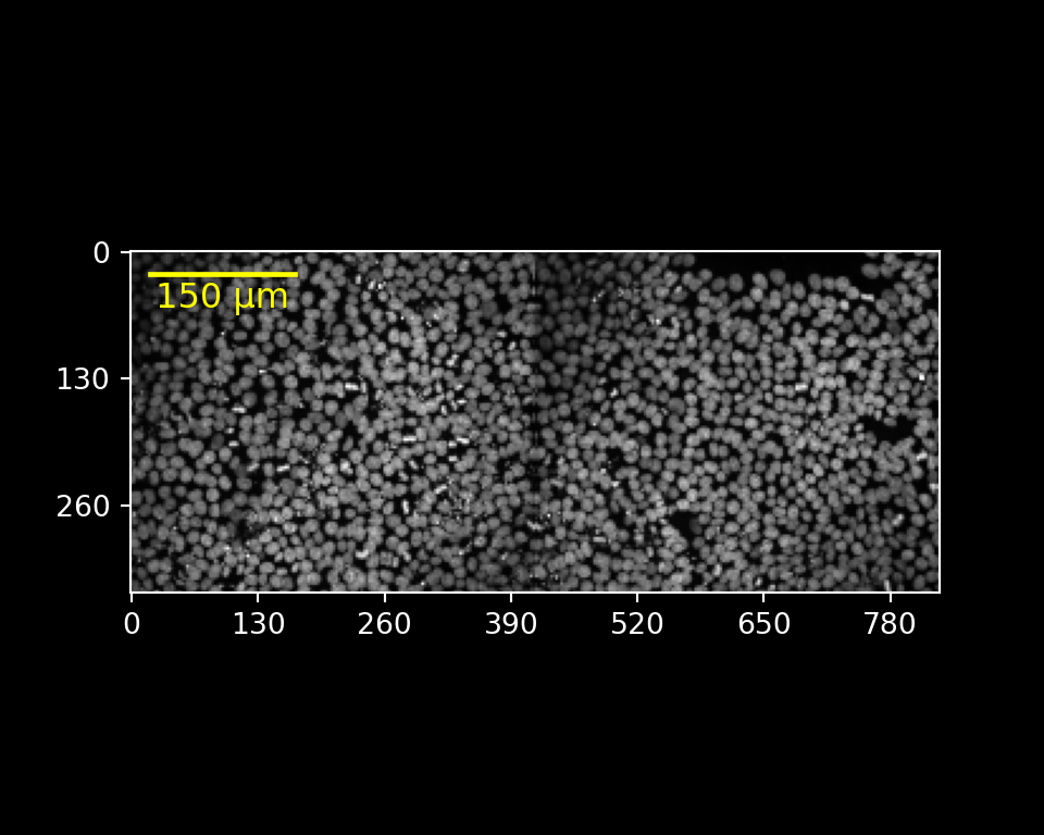

The corresponding R code for interactive is shown below. Please note that you need to use specific R data structures to satisfy the expected arguments types of the python function. For example, a python list ([...]) has to be created using an R list (list(...)) and not a vector. For a list of the conversions that reticulate uses between R and python data structures see reticulate type conversions.

img$plot(channels = list(0L),
         channel_colors = list("white"),
         channel_ranges = list(c(100, 600)),
         scalebar_micrometer = 150L,
         scalebar_color = "yellow",
         scalebar_position = "topleft",
         scalebar_label = TRUE,
         fig_width_inch = 5,
         fig_height_inch = 4,
         fig_dpi = 100,
         axis_style = "micrometer")

Zoom in

r.img.plot(pyramid_level = "0",
           upper_left_yx = [130, 140],
           lower_right_yx = [300, 310],
           scalebar_micrometer = 30,
           scalebar_color = "magenta",
           fig_width_inch = 5,
           fig_height_inch = 5,
           fig_dpi = 100)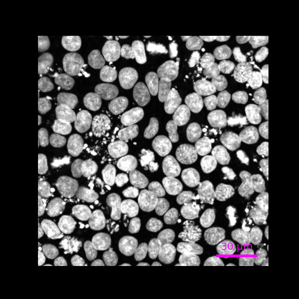

Overlay nuclei segmentation

r.img.plot(label_name = "nuclei", 
           pyramid_level = "0",
           upper_left_yx = [130, 140],
           lower_right_yx = [300, 310],
           scalebar_micrometer = 30,
           scalebar_color = "magenta",
           fig_width_inch = 5,
           fig_height_inch = 5,
           fig_dpi = 100)
#> /Users/runner/Library/Caches/org.R-project.R/R/basilisk/1.21.0/ezzarr/0.1.5/ezzarr/lib/python3.10/site-packages/ez_zarr/ome_zarr.py:929: UserWarning: For the requested pyramid level (0) of the intensity image, no matching label ('nuclei') is available. Up-scaling the label using factor(s) [1. 4. 4.]
#>   warnings.warn(f"For the requested pyramid level ({pyramid_level}) of the intensity image, no matching label ('{lname}') is available. Up-scaling the label using factor(s) {scalefact_yx}")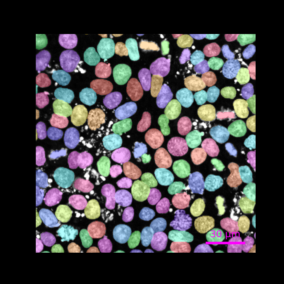

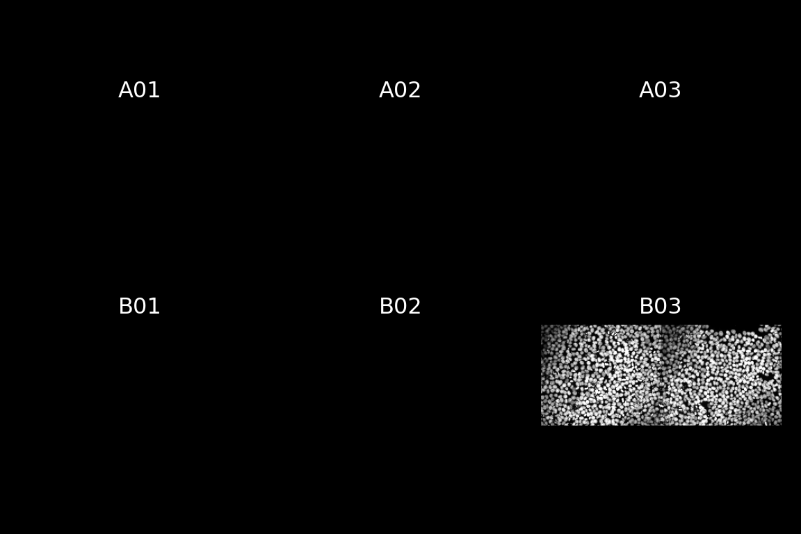
Import and plot entire plate

Above, we imported and visualized a single image. ez-zarr also contains classes to represent high-content screening plates or other, arbitrary, collections of images. Here, we use the import_plate() function to read the whole plate (note that only one well was imaged).

plt <- env$ez_zarr$ome_zarr$import_plate(zarrpath)

Again, we use a python code chunk for the plot to be included in our compiled notebook (not needed for interactive use):

r.plt.plot()

Extract subarray

In addition to plotting, ez-zarr also contains functionality to extract subarrays of a given image, based on coordinates (given either in pixel space for a given pyramid level, or in micrometers). Here we illustrate this by extracting a subarray defined by a bounding box in the x/y plane (the same area that we zoomed in to above), and displaying the resulting array with the EBImage R package.

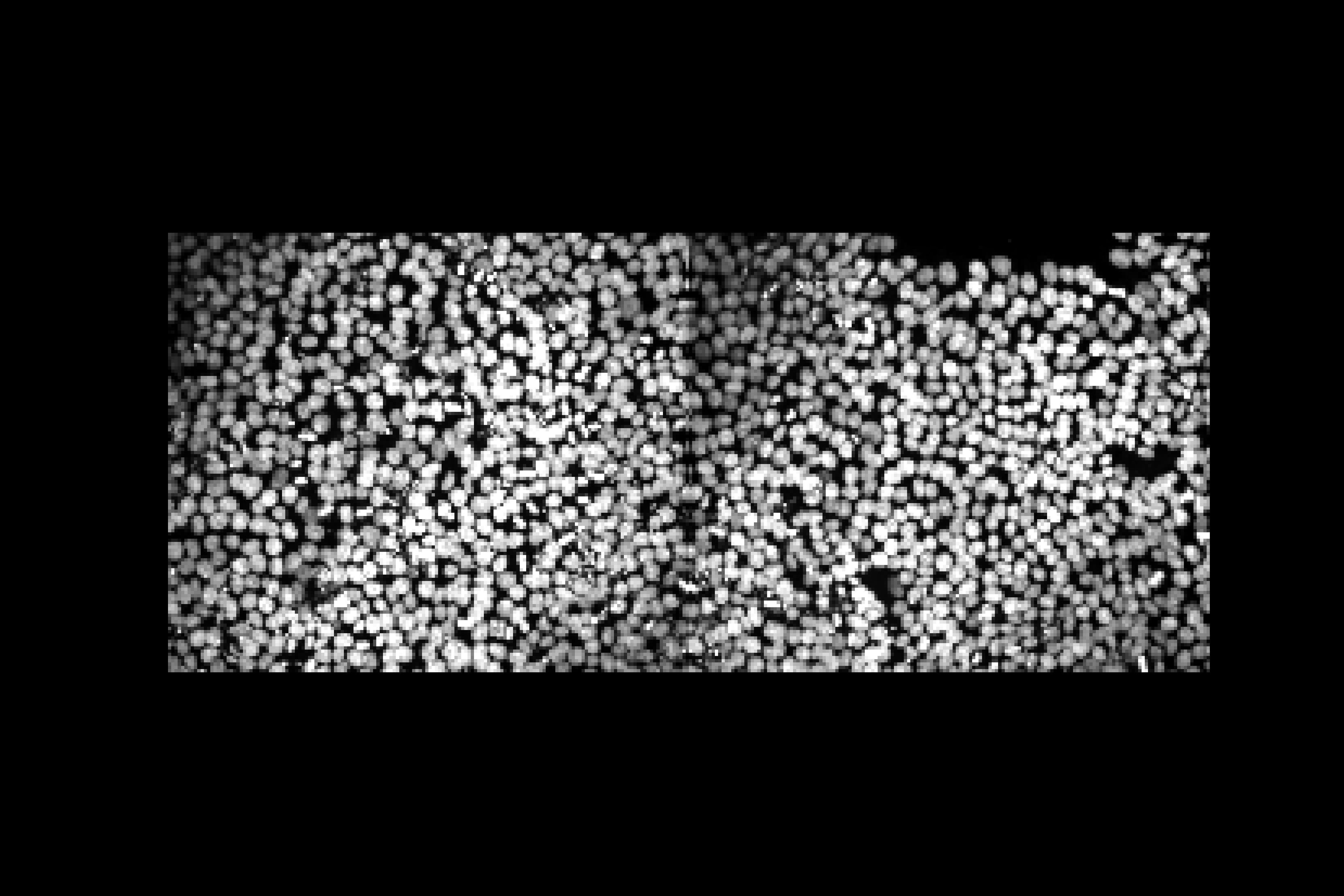
out <- img$get_array_by_coordinate(upper_left_yx = c(130, 140), 
                                   lower_right_yx = c(300, 310), 
                                   pyramid_level = "0", 
                                   as_NumPy = TRUE, 
                                   coordinate_unit = "micrometer")

## Output is an R array
class(out)
#> [1] "array"
dim(out)
#> [1]    1    1 1046 1046

## Display 2d image
im <- EBImage::Image(out[1, 1, , ] / 500)
EBImage::display(im, method = "raster", interpolate = FALSE)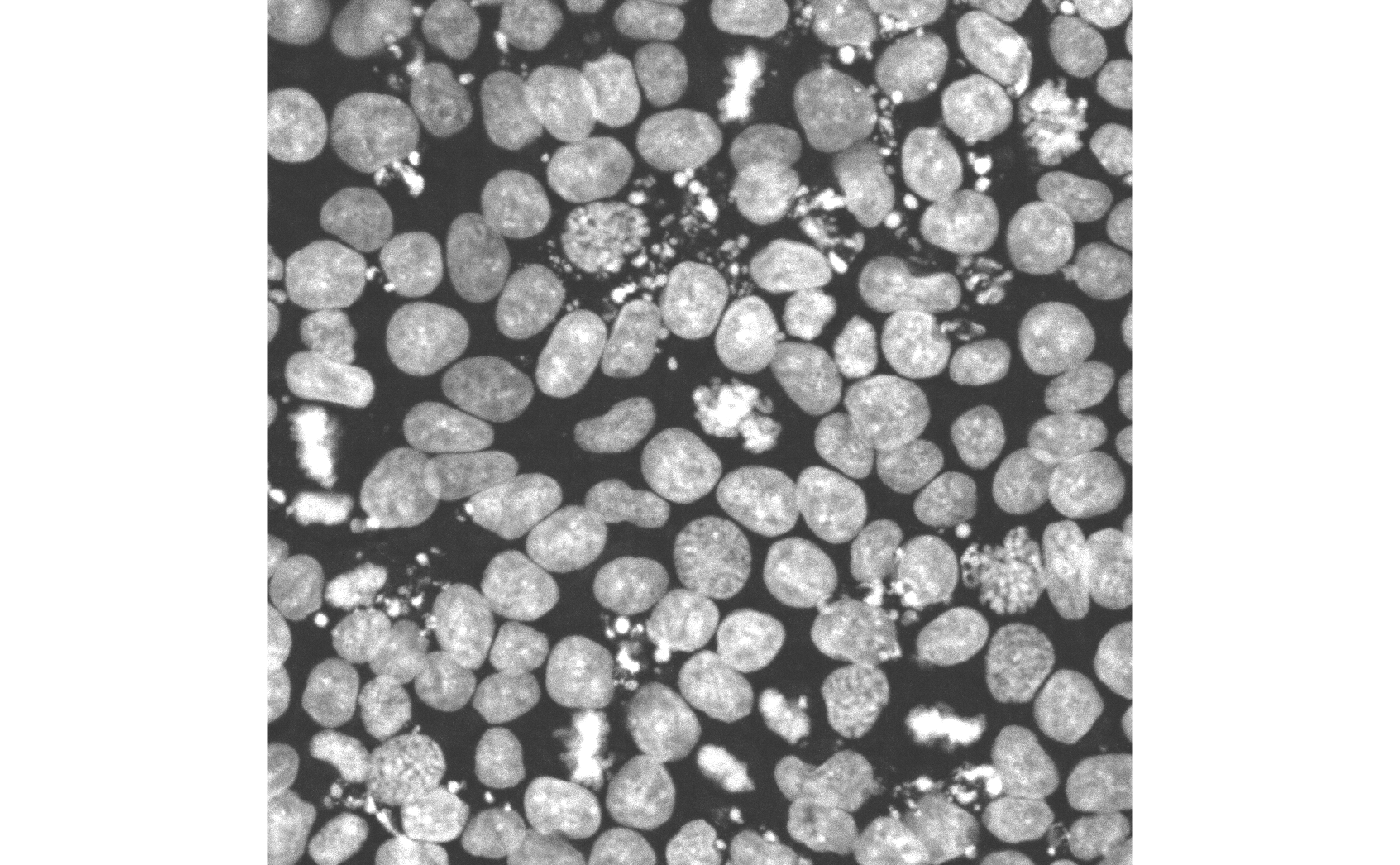

It is also possible to extract a pair of arrays (from the intensity image and one or more of the provided labels).

pair <- img$get_array_pair_by_coordinate(label_name = "nuclei", 
                                         upper_left_yx = c(130, 140),
                                         lower_right_yx = c(300, 310),
                                         pyramid_level = "0",
                                         coordinate_unit = "micrometer")

length(pair)
#> [1] 2

## Intensity image
dim(pair[[1]])
#> [1]    1    1 1044 1048

## Label(s)
length(pair[[2]])
#> [1] 1
dim(pair[[2]][[1]])
#> [1]    1 1044 1048

Session info

sessionInfo()
#> R version 4.5.0 (2025-04-11)
#> Platform: aarch64-apple-darwin20
#> Running under: macOS Sonoma 14.7.5
#> 
#> Matrix products: default
#> BLAS:   /Library/Frameworks/R.framework/Versions/4.5-arm64/Resources/lib/libRblas.0.dylib 
#> LAPACK: /Library/Frameworks/R.framework/Versions/4.5-arm64/Resources/lib/libRlapack.dylib;  LAPACK version 3.12.1
#> 
#> locale:
#> [1] en_US.UTF-8/en_US.UTF-8/en_US.UTF-8/C/en_US.UTF-8/en_US.UTF-8
#> 
#> time zone: UTC
#> tzcode source: internal
#> 
#> attached base packages:
#> [1] stats     graphics  grDevices utils     datasets  methods   base     
#> 
#> other attached packages:
#> [1] EBImage_4.51.0 ezzarr_0.1.5  
#> 
#> loaded via a namespace (and not attached):
#>  [1] Matrix_1.7-3          jsonlite_2.0.0        crayon_1.5.3         
#>  [4] compiler_4.5.0        filelock_1.0.3        Rcpp_1.0.14          
#>  [7] bitops_1.0-9          parallel_4.5.0        jquerylib_0.1.4      
#> [10] systemfonts_1.2.3     textshaping_1.0.1     png_0.1-8            
#> [13] yaml_2.3.10           fastmap_1.2.0         reticulate_1.42.0    
#> [16] lattice_0.22-7        R6_2.6.1              generics_0.1.3       
#> [19] knitr_1.50            BiocGenerics_0.55.0   htmlwidgets_1.6.4    
#> [22] tibble_3.2.1          desc_1.4.3            fftwtools_0.9-11     
#> [25] pillar_1.10.2         bslib_0.9.0           tiff_0.1-12          
#> [28] rlang_1.1.6           cachem_1.1.0          dir.expiry_1.17.0    
#> [31] xfun_0.52             fs_1.6.6              sass_0.4.10          
#> [34] cli_3.6.5             magrittr_2.0.3        withr_3.0.2          
#> [37] pkgdown_2.1.2.9000    digest_0.6.37         grid_4.5.0           
#> [40] locfit_1.5-9.12       basilisk_1.21.0       lifecycle_1.0.4      
#> [43] vctrs_0.6.5           glue_1.8.0            evaluate_1.0.3       
#> [46] ragg_1.4.0            RCurl_1.98-1.17       abind_1.4-8          
#> [49] rmarkdown_2.29        pkgconfig_2.0.3       basilisk.utils_1.21.0
#> [52] tools_4.5.0           jpeg_0.1-11           htmltools_0.5.8.1

Charlotte Soneson, Michael Stadler

2025-05-10

Load the `ezzarr` package

Check the version of ez-zarr

Get the path to the environment

Download example data to temporary directory

Activate the environment

Load an example image

Get details about the image

Plot image

With default settings

Adding a scale bar, limiting the channel range

Zoom in

Overlay nuclei segmentation

Import and plot entire plate

Extract subarray

Session info

Using ez-zarr in R

Charlotte Soneson, Michael Stadler

2025-05-10

Load the ezzarr package

Check the version of ez-zarr

Get the path to the environment

Download example data to temporary directory

Activate the environment

Load an example image

Get details about the image

Plot image

With default settings

Adding a scale bar, limiting the channel range

Zoom in

Overlay nuclei segmentation

Import and plot entire plate

Extract subarray

Session info

Load the `ezzarr` package