Overview
footprintR provides tools for working with
single-molecule footprinting data in R. These include functions for
reading collapsed or read-level data from files generated by Dorado or modkit and
representation of such data as R objects, functions to manipulate such
objects and for visualization.
Current contributors include:
Installation
footprintR can be installed from GitHub via the
BiocManager package:
if (!requireNamespace("BiocManager", quietly = TRUE))
    install.packages("BiocManager")

BiocManager::install("fmicompbio/footprintR")
Functionality
Here is a minimal example for using footprintR that
illustrates its functionality using summary-level data.
We start by loading the package:
Read summary data from bed files
Here, we will demonstrate how to read and visualize summary-level
data (where individual reads have been combined per genomic position).
For an example of how to work with read-level data, see the
vignette("read-level-data").
The example is using small example data provided as part of the
package. Here we get the file names for per-position summary
modification data in bedMethyl format:
# collapsed 5mC data for a small genomic window in bedMethyl format
bedmethylfiles <- system.file("extdata",
                              c("modkit_pileup_1.bed.gz",
                                "modkit_pileup_2.bed.gz"),
                              package = "footprintR")

# file with sequence of the reference genome in fasta format
reffile <- system.file("extdata", "reference.fa.gz", package = "footprintR")
This allows us to read the data using
readBedMethyl():
names(bedmethylfiles) <- c("sample1", "sample2")
se <- readBedMethyl(bedmethylfiles,
                    sequence.context = 3,
                    sequence.reference = reffile)
se
#> class: RangedSummarizedExperiment
#> dim: 12020 2
#> metadata(0):
#> assays(2): Nmod Nvalid
#> rownames: NULL
#> rowData names(1): sequence.context
#> colnames(2): sample1 sample2
#> colData names(0):
These bedMethyl files contain summarized data and are
read into a RangedSummarizedExperiment object. The rows
here correspond to genomic positions:
rowRanges(se)
#> UnstitchedGPos object with 12020 positions and 1 metadata column:
#>           seqnames       pos strand | sequence.context
#>              <Rle> <integer>  <Rle> |   <DNAStringSet>
#>       [1]     chr1   6937686      + |              GCA
#>       [2]     chr1   6937688      + |              ACT
#>       [3]     chr1   6937689      + |              CTT
#>       [4]     chr1   6937691      + |              TAA
#>       [5]     chr1   6937696      + |              GCA
#>       ...      ...       ...    ... .              ...
#>   [12016]     chr1   6957049      - |              TGG
#>   [12017]     chr1   6957051      - |              CCT
#>   [12018]     chr1   6957052      - |              TCC
#>   [12019]     chr1   6957056      - |              CCT
#>   [12020]     chr1   6957057      - |              CCC
#>   -------
#>   seqinfo: 1 sequence from an unspecified genome; no seqlengths
… and the columns correspond to the different samples (here
corresponding to the names of the two input files in
bedmethylfiles):
colnames(se)
#> [1] "sample1" "sample2"
The data is stored in two matrices (assays) called Nmod
(the number of modified bases per sample and position) and
Nvalid (the number of valid total read covering that
position in each sample):
assayNames(se)
#> [1] "Nmod"   "Nvalid"

head(assay(se, "Nmod"))
#>      sample1 sample2
#> [1,]       1       5
#> [2,]       1       0
#> [3,]       0       0
#> [4,]       0       0
#> [5,]       3       3
#> [6,]       0       0
head(assay(se, "Nvalid"))
#>      sample1 sample2
#> [1,]      16      15
#> [2,]      16      15
#> [3,]       0       1
#> [4,]       1       0
#> [5,]      16      14
#> [6,]       1       0
From these, you can easily calculate the fraction of modifications:
fraction_modified <- assay(se, "Nmod") / assay(se, "Nvalid")
head(fraction_modified)
#>      sample1   sample2
#> [1,]  0.0625 0.3333333
#> [2,]  0.0625 0.0000000
#> [3,]     NaN 0.0000000
#> [4,]  0.0000       NaN
#> [5,]  0.1875 0.2142857
#> [6,]  0.0000       NaN
Please note that non-finite fractions result from positions that had zero coverage in a given sample.
Plot data
Use the plotRegion() function to visualize data for a
specific region, here visualizing the accessibility using GpC
methylation (sequence context GCH), and adding a smooth line:
plotRegion(se,
           region = "chr1:6939000-6946000",
           tracks.summary = list(FracMod = "PointSmooth"),
           sequence.context = "GCH")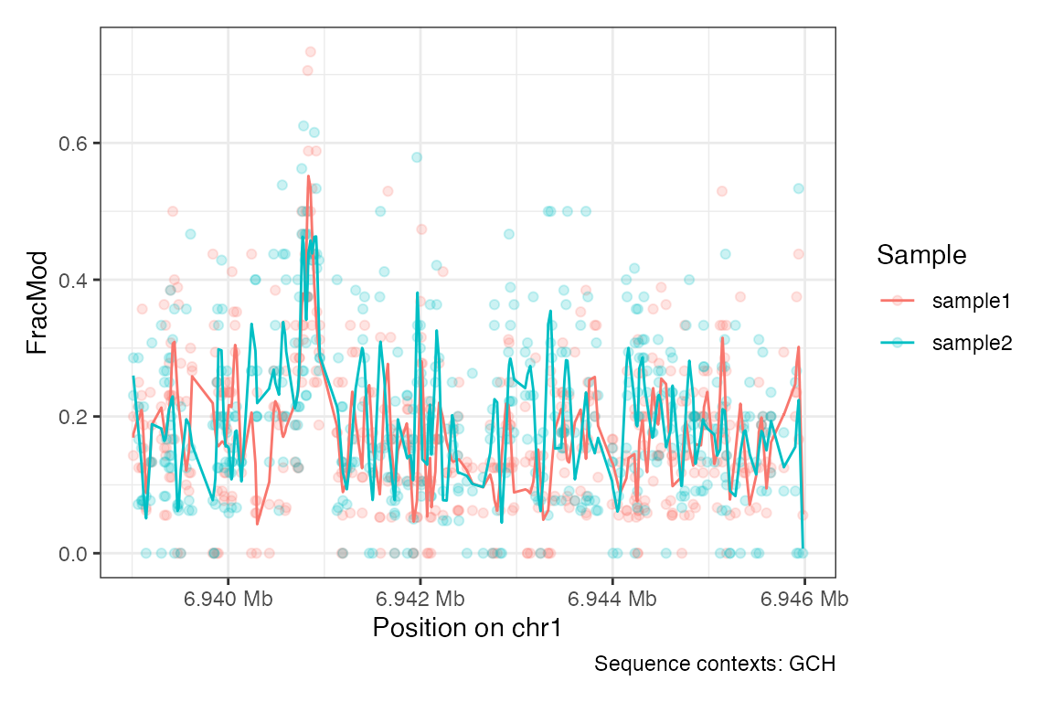
Or the endogenous DNA methylation (sequence context HCG):
plotRegion(se,
           region = "chr1:6939000-6946000",
           tracks.summary = list(FracMod = "PointSmooth"),
           sequence.context = "HCG")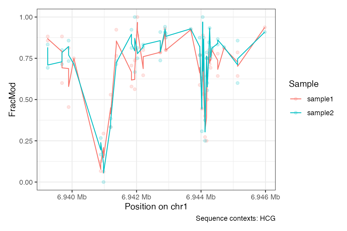
Or just plotting the coverage (Nvalid) as a smooth
line:
plotRegion(se,
           region = "chr1:6939000-6946000",
           tracks.summary = list(Nvalid = "Smooth"))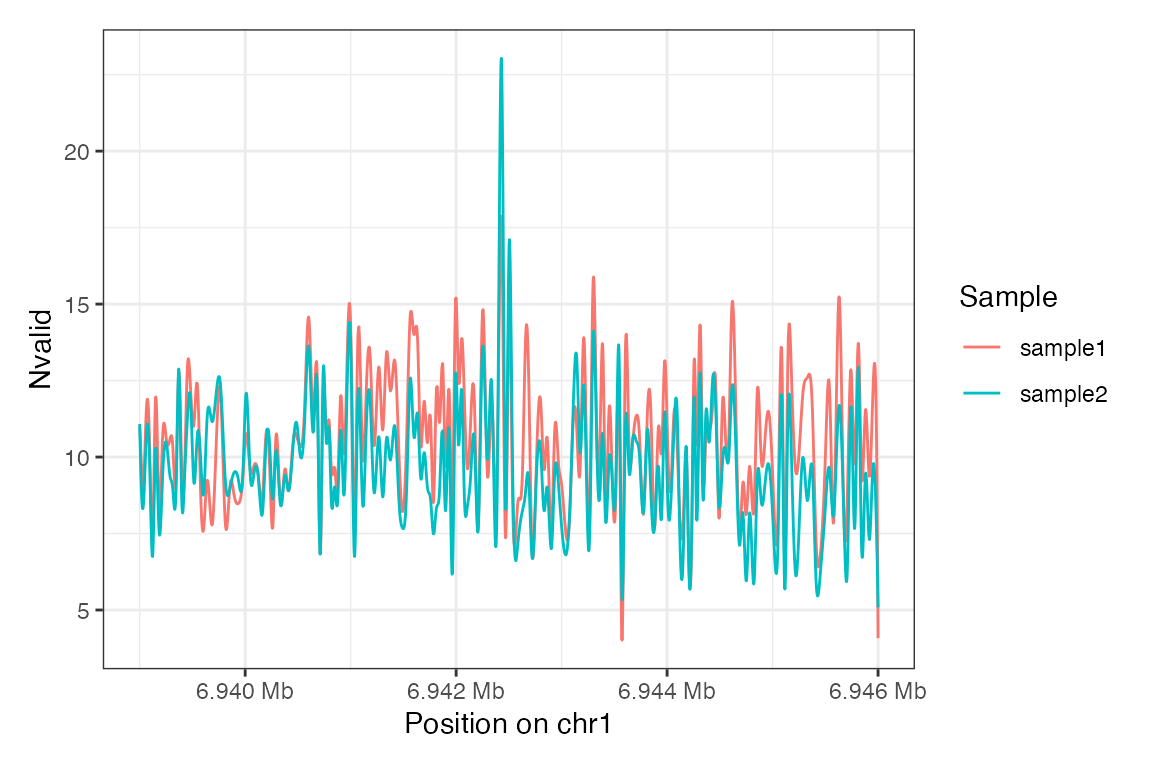
Session info
sessionInfo()
#> R version 4.4.1 (2024-06-14)
#> Platform: aarch64-apple-darwin20
#> Running under: macOS Sonoma 14.6.1
#>
#> Matrix products: default
#> BLAS:   /Library/Frameworks/R.framework/Versions/4.4-arm64/Resources/lib/libRblas.0.dylib
#> LAPACK: /Library/Frameworks/R.framework/Versions/4.4-arm64/Resources/lib/libRlapack.dylib;  LAPACK version 3.12.0
#>
#> locale:
#> [1] en_US.UTF-8/en_US.UTF-8/en_US.UTF-8/C/en_US.UTF-8/en_US.UTF-8
#>
#> time zone: UTC
#> tzcode source: internal
#>
#> attached base packages:
#> [1] stats4    stats     graphics  grDevices utils     datasets  methods
#> [8] base
#>
#> other attached packages:
#>  [1] SummarizedExperiment_1.35.1 Biobase_2.65.1
#>  [3] GenomicRanges_1.57.1        GenomeInfoDb_1.41.1
#>  [5] IRanges_2.39.2              S4Vectors_0.43.2
#>  [7] BiocGenerics_0.51.1         MatrixGenerics_1.17.0
#>  [9] matrixStats_1.4.1           footprintR_0.1.2
#>
#> loaded via a namespace (and not attached):
#>  [1] tidyselect_1.2.1            dplyr_1.1.4
#>  [3] farver_2.1.2                R.utils_2.12.3
#>  [5] Biostrings_2.73.1           bitops_1.0-8
#>  [7] fastmap_1.2.0               SingleCellExperiment_1.27.2
#>  [9] RCurl_1.98-1.16             GenomicAlignments_1.41.0
#> [11] XML_3.99-0.17               digest_0.6.37
#> [13] lifecycle_1.0.4             magrittr_2.0.3
#> [15] compiler_4.4.1              rlang_1.1.4
#> [17] sass_0.4.9                  tools_4.4.1
#> [19] utf8_1.2.4                  yaml_2.3.10
#> [21] data.table_1.16.0           rtracklayer_1.65.0
#> [23] knitr_1.48                  labeling_0.4.3
#> [25] S4Arrays_1.5.7              curl_5.2.2
#> [27] DelayedArray_0.31.11        abind_1.4-8
#> [29] BiocParallel_1.39.0         withr_3.0.1
#> [31] purrr_1.0.2                 desc_1.4.3
#> [33] R.oo_1.26.0                 grid_4.4.1
#> [35] fansi_1.0.6                 beachmat_2.21.6
#> [37] colorspace_2.1-1            ggplot2_3.5.1
#> [39] scales_1.3.0                cli_3.6.3
#> [41] rmarkdown_2.28              crayon_1.5.3
#> [43] ragg_1.3.3                  generics_0.1.3
#> [45] httr_1.4.7                  rjson_0.2.23
#> [47] scuttle_1.15.4              cachem_1.1.0
#> [49] zlibbioc_1.51.1             parallel_4.4.1
#> [51] XVector_0.45.0              restfulr_0.0.15
#> [53] vctrs_0.6.5                 Matrix_1.7-0
#> [55] jsonlite_1.8.8              patchwork_1.3.0
#> [57] systemfonts_1.1.0           jquerylib_0.1.4
#> [59] tidyr_1.3.1                 glue_1.7.0
#> [61] pkgdown_2.1.0.9000          codetools_0.2-20
#> [63] gtable_0.3.5                BiocIO_1.15.2
#> [65] UCSC.utils_1.1.0            munsell_0.5.1
#> [67] tibble_3.2.1                pillar_1.9.0
#> [69] htmltools_0.5.8.1           GenomeInfoDbData_1.2.12
#> [71] BSgenome_1.73.1             R6_2.5.1
#> [73] textshaping_0.4.0           evaluate_1.0.0
#> [75] lattice_0.22-6              highr_0.11
#> [77] R.methodsS3_1.8.2           Rsamtools_2.21.1
#> [79] bslib_0.8.0                 Rcpp_1.0.13
#> [81] SparseArray_1.5.34          xfun_0.47
#> [83] fs_1.6.4                    pkgconfig_2.0.3