einprot
2026-03-12
einprot.Rmd
library(S4Vectors)
library(SummarizedExperiment)
library(einprot)
Introduction
The einprot R package provides easy-to-use end-to-end
proteomics workflows for data quantified with either
MaxQuant (Cox and Mann 2008)
(LFQ), Proteome Discoverer (Orsburn
2021) (TMT), or FragPipe. It was
originally developed to support the proteomics platform at the FMI. The
package can be installed from GitHub as follows:
install.packages("remotes")
remotes::install_github("fmicompbio/einprot")
Running a full workflow
The main functions for running an end-to-end workflow are (depending on the experiment type and quantification engine)
Each of these functions takes a set of arguments defining input files
as well as analysis parameters, injects these into an R markdown
template, and renders the resulting .Rmd file into an html report. In
the process, a collection of output files are generated, including lists
and plots of differentially abundant proteins, and a final
SingleCellExperiment object for further exploration and
analysis.
As an example, we will illustrate how to run the
MaxQuant workflow using the example data provided in
einprot (from Ostapcuk et al.
(2018)). The process is similar for the other workflows. The
MaxQuant workflow requires a MaxQuant
proteinGroups.txt file as well as (optionally) the XML
parameter file. The type of intensities to use for the analysis is
specified via the iColPattern argument. The following code
runs the workflow, using mostly default parameter values:
(sampleAnnot <- read.delim(system.file("extdata", "mq_example", "1356_sampleAnnot.txt",
                                       package = "einprot")))
out <- runMaxQuantAnalysis(
    outputDir = tempdir(),
    outputBaseName = "MQ_LFQ",
    reportTitle = "MaxQuant LFQ data processing",
    reportAuthor = "Charlotte Soneson",
    species = "mouse",
    mqFile = system.file("extdata", "mq_example", "1356_proteinGroups.txt",
                         package = "einprot"),
    mqParameterFile = system.file("extdata", "mq_example", "1356_mqpar.xml",
                                  package = "einprot"),
    iColPattern = "^LFQ\\.intensity\\.",
    sampleAnnot = sampleAnnot,
    imputeMethod = "MinProb",
    ctrlGroup = "RBC_ctrl",
    allPairwiseComparisons = FALSE,
    normMethod = "none",
    stattest = "limma",
    includeFeatureCollections = "complexes"
)
This run will generate a collection of output files in the designated
output directory (here, a temporary directory). All files will be named
with the prefix specified by outputBaseName.
Output files generated by the workflows
Running the einprot workflow above will generate the
following set of output files in the designated output directory:
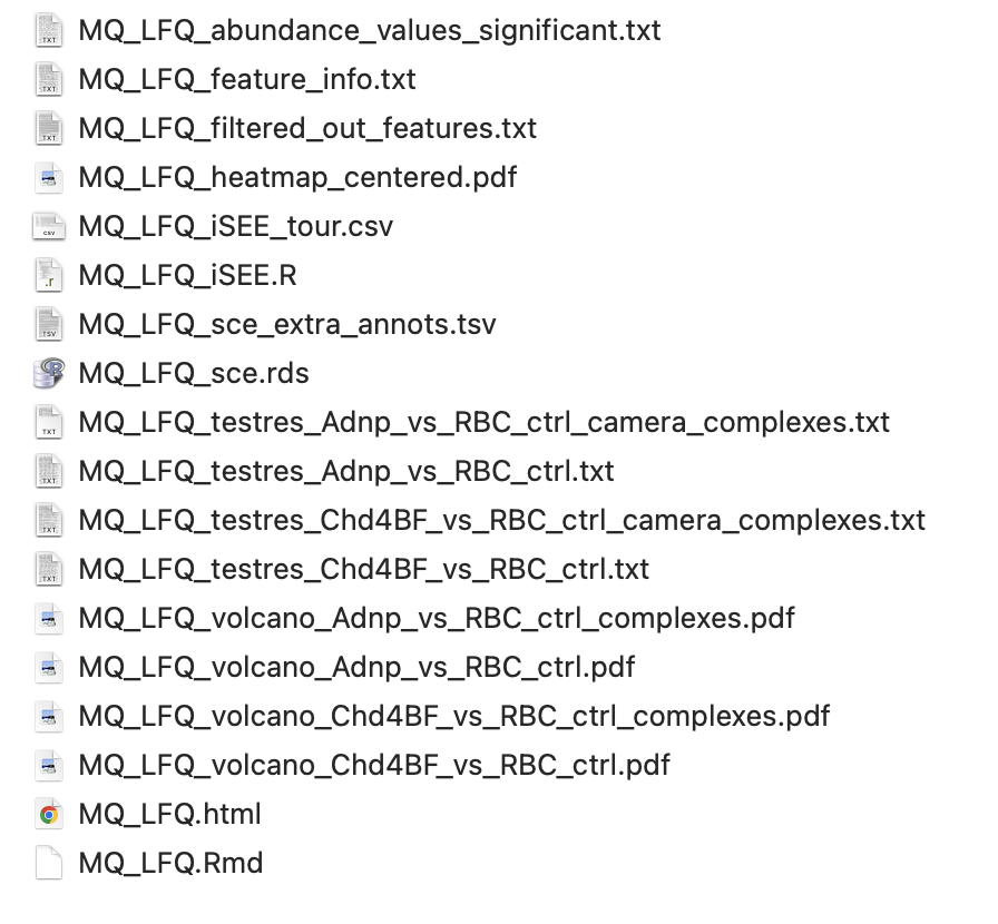
- A self-contained .Rmd file (here,
MQ_LFQ.Rmd) with all the code run in the workflow. In principle, this can be edited and rerun manually. Note, however, that if the workflow function is called again, the file will be overwritten (ifforceOverwriteargument is set toTRUE). - An html report (
MQ_LFQ.html) obtained by rendering the .Rmd file. - A
SingleCellExperimentobject serialized to an .rds file (MQ_LFQ_sce.rds). This object reflects all the analysis steps of the workflow, and is exported at the end of rendering the .Rmd file. Very long annotation columns are stored in a separate file (MQ_LFQ_sce_extra_annots.tsv). - Result files from the differential expression analysis, both for
individual proteins and for feature sets (known protein complexes and/or
GO terms, if applicable) (
MQ_LFQ_testres_*.txt), and exported abundance values for all significant features (MQ_LFQ_abundance_values_significant.txt). - pdf files with volcano plots for differential abundance analysis
(
MQ_LFQ_volcano_*.pdf), and a heatmap of the overall abundance matrix (MQ_LFQ_heatmap_centered.pdf, only for theMaxQuantandFragPipeworkflows). - An R script that, when sourced, will launch an adapted
iSEE(Rue-Albrecht et al. 2018) session for interactive exploration of the data (MQ_LFQ_iSEE.R, which incorporates an interactive guided tour specified inMQ_LFQ_iSEE_tour.csv). - Additional information about retained and filtered-out features
(
MQ_LFQ_feature_info.txt,MQ_LFQ_filtered_out_features.txt).
All file names start with the outputBaseName specified
in the call to runMaxQuantAnalysis (here,
MQ_LFQ).
Listing supported species
The list of species currently supported by einprot can
be obtained using the function getSupportedSpecies(). The
species information is used to retrieve suitable feature identifiers for
complexes and GO terms (if requested), and to provide automatic links to
species-specific databases such as PomBase and WormBase, whenever
applicable.
getSupportedSpecies()
#>     taxId                         species        speciesCommon
#> 1   10090                    Mus musculus                mouse
#> 2    9606                    Homo sapiens                human
#> 3    6239          Caenorhabditis elegans            roundworm
#> 4    7955                     Danio rerio            zebrafish
#> 5    7227         Drosophila melanogaster             fruitfly
#> 6    4932        Saccharomyces cerevisiae        baker's yeast
#> 7  284812 Schizosaccharomyces pombe 972h-        fission yeast
#> 8   28377             Anolis carolinensis          green anole
#> 9    9913                      Bos taurus               bovine
#> 10   9615          Canis lupus familiaris                  dog
#> 11   9796                  Equus caballus                horse
#> 12   9685                     Felis catus                  cat
#> 13   9031                   Gallus gallus              chicken
#> 14   9544                  Macaca mulatta       rhesus macaque
#> 15  13616           Monodelphis domestica              opossum
#> 16   9258        Ornithorhynchus anatinus             platypus
#> 17   9598                 Pan troglodytes           chimpanzee
#> 18  10116               Rattus norvegicus           Norway rat
#> 19   9823                      Sus scrofa                  pig
#> 20   8364              Xenopus tropicalis tropical clawed frog
Listing available complex DBs
If specified by the user, einprot will test for
differential abundance not only of individual proteins, but also of
feature sets. Currently, GO terms and protein complexes (plus any
user-specified sets) are supported. The built-in complex database was
created using the makeComplexDB() function, and combines
annotated complexes for multiple different species. Regardless of where
it was originally defined, each complex is also lifted over to the
current species of interest, using the ortholog conversion functionality
of the babelgene package. To list the available complex
databases provided by einprot, we can use the
listComplexDBs() function:
## List available complex databases
(lcdb <- listComplexDBs())
#>                                                                                              complexDbPath
#> 1 /Users/runner/work/_temp/Library/einprot/extdata/complexes/complexdb_einprot0.9.3_20240328_orthologs.rds
#> 2 /Users/runner/work/_temp/Library/einprot/extdata/complexes/complexdb_einprot0.5.0_20220323_orthologs.rds
#>      genDate
#> 1 2024-03-28
#> 2 2022-03-23

## Read the most recent one
cdb <- readRDS(lcdb$complexDbPath[1])

## cdb is a list of databases - each one containing identifiers for a
## specific species
class(cdb)
#> [1] "list"
names(cdb)
#> [1] "mouse"                           "human"
#> [3] "baker's yeast"                   "Caenorhabditis elegans"
#> [5] "Schizosaccharomyces pombe 972h-"

cdb$mouse
#> CharacterList of length 11257
#> [["mouse: (ER)-localized multiprotein complex, Ig heavy chains associated"]] ...
#> [["mouse: (ER)-localized multiprotein complex, in absence of Ig heavy chains"]]
#> [["mouse: 20S proteasome"]] Psmb1 Psmb5 Psma3 Psma2 ... Psmb2 Psma1 Psma7 Psma5
#> [["mouse: A2m-Anxa6-Lrp1 complex"]] A2M ANXA6 Anxa6 LRP1 A2m Lrp1
#> [["mouse: Abcg5-Abcg1 complex"]] Abcg1 Abcg5
#> [["mouse: Abcg5-Abcg2 complex"]] Abcg2 Abcg5
#> [["mouse: Abcg5-Abcg4 complex"]] Abcg4 Abcg5
#> [["mouse: Abcg5-Abcg8 complex (+1 alt. ID)"]] Abcg5 Abcg8
#> [["mouse: Abcg8-Abcg4 complex"]] Abcg4 Abcg8
#> [["mouse: Abi1-Wasl complex (+1 alt. ID)"]] Abi1 Wasl
#> ...
#> <11247 more elements>

## Additional information about the complexes
mcols(cdb$mouse)
#> DataFrame with 11257 rows and 4 columns
#>                                                                           Species.common
#>                                                                              <character>
#> mouse: (ER)-localized multiprotein complex, Ig heavy chains associated             mouse
#> mouse: (ER)-localized multiprotein complex, in absence of Ig heavy chains          mouse
#> mouse: 20S proteasome                                                              mouse
#> mouse: A2m-Anxa6-Lrp1 complex                                                      mouse
#> mouse: Abcg5-Abcg1 complex                                                         mouse
#> ...                                                                                  ...
#> S.pombe: vacuolar proton-transporting V-type ATPase, V1 domain             Schizosacc...
#> S.pombe: voltage-gated potassium channel complex                           Schizosacc...
#> S.pombe: Vps55/Vps68 complex                                               Schizosacc...
#> S.pombe: Wpl/Pds5 cohesin loading/unloading complex                        Schizosacc...
#> S.pombe: zeta DNA polymerase complex                                       Schizosacc...
#>                                                                                Source
#>                                                                           <character>
#> mouse: (ER)-localized multiprotein complex, Ig heavy chains associated          CORUM
#> mouse: (ER)-localized multiprotein complex, in absence of Ig heavy chains       CORUM
#> mouse: 20S proteasome                                                           CORUM
#> mouse: A2m-Anxa6-Lrp1 complex                                                   CORUM
#> mouse: Abcg5-Abcg1 complex                                                      CORUM
#> ...                                                                               ...
#> S.pombe: vacuolar proton-transporting V-type ATPase, V1 domain                pombase
#> S.pombe: voltage-gated potassium channel complex                              pombase
#> S.pombe: Vps55/Vps68 complex                                                  pombase
#> S.pombe: Wpl/Pds5 cohesin loading/unloading complex                           pombase
#> S.pombe: zeta DNA polymerase complex                                          pombase
#>                                                                                    PMID
#>                                                                             <character>
#> mouse: (ER)-localized multiprotein complex, Ig heavy chains associated         12475965
#> mouse: (ER)-localized multiprotein complex, in absence of Ig heavy chains      12475965
#> mouse: 20S proteasome                                                          10436176
#> mouse: A2m-Anxa6-Lrp1 complex                                                  15226301
#> mouse: Abcg5-Abcg1 complex                                                     14504269
#> ...                                                                                 ...
#> S.pombe: vacuolar proton-transporting V-type ATPase, V1 domain            14735354;G...
#> S.pombe: voltage-gated potassium channel complex                          GO_REF:000...
#> S.pombe: Vps55/Vps68 complex                                              GO_REF:000...
#> S.pombe: Wpl/Pds5 cohesin loading/unloading complex                            26687354
#> S.pombe: zeta DNA polymerase complex                                      GO_REF:000...
#>                                                                               All.names
#>                                                                             <character>
#> mouse: (ER)-localized multiprotein complex, Ig heavy chains associated    mouse: (ER...
#> mouse: (ER)-localized multiprotein complex, in absence of Ig heavy chains mouse: (ER...
#> mouse: 20S proteasome                                                     mouse: 20S...
#> mouse: A2m-Anxa6-Lrp1 complex                                             mouse: A2m...
#> mouse: Abcg5-Abcg1 complex                                                mouse: Abc...
#> ...                                                                                 ...
#> S.pombe: vacuolar proton-transporting V-type ATPase, V1 domain            S.pombe: v...
#> S.pombe: voltage-gated potassium channel complex                          S.pombe: v...
#> S.pombe: Vps55/Vps68 complex                                              S.pombe: V...
#> S.pombe: Wpl/Pds5 cohesin loading/unloading complex                       S.pombe: W...
#> S.pombe: zeta DNA polymerase complex                                      S.pombe: z...
Checking the intensity column pattern
As described above, the workflow functions require the specification
of a ‘column pattern’, that determines which columns will be extracted
from the input text file to generate the main intensity matrix. To check
which columns will be extracted with a given column pattern, we can use
the getIntensityColumns() function, provided with the path
to the input text file and the desired iColPattern.
mqFile <- system.file("extdata", "mq_example", "1356_proteinGroups.txt",
                      package = "einprot")
getIntensityColumns(inFile = mqFile, iColPattern = "^LFQ\\.intensity\\.")
#> $iColsAll
#> [1] "LFQ.intensity.Adnp_IP04"     "LFQ.intensity.Adnp_IP05"
#> [3] "LFQ.intensity.Adnp_IP06"     "LFQ.intensity.Chd4BF_IP07"
#> [5] "LFQ.intensity.Chd4BF_IP08"   "LFQ.intensity.Chd4BF_IP09"
#> [7] "LFQ.intensity.RBC_ctrl_IP01" "LFQ.intensity.RBC_ctrl_IP02"
#> [9] "LFQ.intensity.RBC_ctrl_IP03"
#>
#> $iCols
#> [1] "LFQ.intensity.Adnp_IP04"     "LFQ.intensity.Adnp_IP05"
#> [3] "LFQ.intensity.Adnp_IP06"     "LFQ.intensity.Chd4BF_IP07"
#> [5] "LFQ.intensity.Chd4BF_IP08"   "LFQ.intensity.Chd4BF_IP09"
#> [7] "LFQ.intensity.RBC_ctrl_IP01" "LFQ.intensity.RBC_ctrl_IP02"
#> [9] "LFQ.intensity.RBC_ctrl_IP03"
Reading data into a SingleCellExperiment object
einprot contains functionality for reading data from
MaxQuant, FragPipe and
ProteomeDiscoverer protein quantification text files and
generating a SingleCellExperiment object. All columns in
the text file that are typically sample-specific will be converted into
assays, while all other columns will be added as row annotations.
imp <- importExperiment(mqFile, iColPattern = "^LFQ\\.intensity\\.")

## The aName output provides the name of the "main" assay
## (corresponding to the specified iColPattern)
imp$aName
#> [1] "LFQ.intensity"

## Imported SingleCellExperiment object
imp$sce
#> class: SingleCellExperiment
#> dim: 463 9
#> metadata(1): colList
#> assays(9): LFQ.intensity MS.MS.Count ... iBAQ Identification.type
#> rownames(463): 1 2 ... 462 463
#> rowData names(35): Protein.IDs Majority.protein.IDs ...
#>   Oxidation.M.site.IDs Oxidation.M.site.positions
#> colnames(9): Adnp_IP04 Adnp_IP05 ... RBC_ctrl_IP02 RBC_ctrl_IP03
#> colData names(0):
#> reducedDimNames(0):
#> mainExpName: NULL
#> altExpNames(0):

## All assays
assayNames(imp$sce)
#> [1] "LFQ.intensity"         "MS.MS.Count"           "Intensity"
#> [4] "Sequence.coverage"     "Unique.peptides"       "Razor.unique.peptides"
#> [7] "Peptides"              "iBAQ"                  "Identification.type"

## Row annotation
rowData(imp$sce)
#> DataFrame with 463 rows and 35 columns
#>       Protein.IDs Majority.protein.IDs Peptide.counts.all
#>       <character>          <character>        <character>
#> 1   A0A023T672...        A0A023T672...              1;1;1
#> 2   A0A087WPL5...        A0A087WPL5...      13;13;11;1...
#> 3   Q3UH28;Q3U...        Q3UH28;Q3U...      3;3;3;3;3;...
#> 4   A2A513;CON...        A2A513;CON...      14;14;14;1...
#> 5   A2A791;A2A...        A2A791;A2A...           56;55;44
#> ...           ...                  ...                ...
#> 459 REV__P2873...        REV__P2873...                  1
#> 460 REV__P5871...        REV__P5871...                  1
#> 461 REV__Q8BHW...        REV__Q8BHW...                  1
#> 462 V9GWW1;Q68...        V9GWW1;Q68...      42;40;27;2...
#> 463        V9GXP2               V9GXP2                 29
#>     Peptide.counts.razor.unique Peptide.counts.unique Protein.names
#>                     <character>           <character>   <character>
#> 1                         1;1;1                 1;1;1 RNA-bindin...
#> 2                 13;13;11;1...         13;13;11;1... ATP-depend...
#> 3                 3;3;3;3;3;...         3;3;3;3;3;...
#> 4                     1;1;1;1;1             1;1;1;1;1 Keratin, t...
#> 5                      56;55;44              56;55;44 Zinc finge...
#> ...                         ...                   ...           ...
#> 459                           1                     1
#> 460                           1                     1
#> 461                           1                     1
#> 462               42;40;27;2...         12;10;0;1;... Zinc finge...
#> 463                           2                     1
#>        Gene.names Fasta.headers Number.of.proteins  Peptides
#>       <character>   <character>          <integer> <integer>
#> 1      RBM8;Rbm8a >tr|A0A023...                  3         1
#> 2            Dhx9 >tr|A0A087...                  6        13
#> 3          Zmynd8 >tr|Q3UH28...                  7         3
#> 4           Krt10 >tr|A2A513...                  5        14
#> 5           Zmym4 >sp|A2A791...                  3        56
#> ...           ...           ...                ...       ...
#> 459               >sp|P28738...                  1         1
#> 460               >sp|P58710...                  1         1
#> 461               >sp|Q8BHW5...                  1         1
#> 462 Zfp280d;Zn... >tr|V9GWW1...                 10        42
#> 463       Zfp280d >tr|V9GXP2...                  1        29
#>     Razor.unique.peptides Unique.peptides Sequence.coverage
#>                 <integer>       <integer>         <numeric>
#> 1                       1               1              10.9
#> 2                      13              13              13.1
#> 3                       3               3               3.6
#> 4                       1               1              18.7
#> 5                      56              56              48.7
#> ...                   ...             ...               ...
#> 459                     1               1               0.0
#> 460                     1               1               0.0
#> 461                     1               1               0.0
#> 462                    42              12              62.3
#> 463                     2               1              52.6
#>     Unique.razor.sequence.coverage Unique.sequence.coverage Mol.weight.kDa
#>                          <numeric>                <numeric>      <numeric>
#> 1                             10.9                     10.9         19.889
#> 2                             13.1                     13.1        149.620
#> 3                              3.6                      3.6        127.290
#> 4                              3.4                      3.4         57.040
#> 5                             48.7                     48.7        172.440
#> ...                            ...                      ...            ...
#> 459                            0.0                      0.0        109.270
#> 460                            0.0                      0.0         50.478
#> 461                            0.0                      0.0         36.570
#> 462                           62.3                     20.5        104.870
#> 463                            3.0                      1.5         90.174
#>     Sequence.length Sequence.lengths   Q.value     Score  Intensity      iBAQ
#>           <integer>      <character> <numeric> <numeric>  <numeric> <numeric>
#> 1               174    174;173;17... 0.0000000   15.2130   34384000   4298000
#> 2              1383    1383;1384;... 0.0000000   35.8400  156100000   2477800
#> 3              1154    1154;1174;... 0.0000000   44.9200   28924000    490240
#> 4               561    561;570;46... 0.0027174    4.5113   29053000   1117400
#> 5              1549    1549;1460;... 0.0000000  323.3100 2787500000  39822000
#> ...             ...              ...       ...       ...        ...       ...
#> 459             956              956 1.0000000   -2.0000   97210000       NaN
#> 460             440              440 0.0100760    3.6649 4734200000       NaN
#> 461             331              331 1.0000000   -2.0000  349630000       NaN
#> 462             949    949;974;78... 0.0000000  323.3100 3057000000  66457000
#> 463             799              799 0.0027322    4.6147   46397000   1104700
#>     MS.MS.Count Only.identified.by.site     Reverse Potential.contaminant
#>       <integer>             <character> <character>           <character>
#> 1             7
#> 2            25
#> 3            10
#> 4             5                                                         +
#> 5           195
#> ...         ...                     ...         ...                   ...
#> 459           1                       +           +
#> 460          19                                   +
#> 461           5                       +           +
#> 462         148
#> 463           2
#>            id   Peptide.IDs Peptide.is.razor Mod.peptide.IDs  Evidence.IDs
#>     <integer>   <character>      <character>     <character>   <character>
#> 1           0          2965             True            3291 21752;2175...
#> 2           1 13;191;192...    True;True;...   14;213;214... 33;34;35;3...
#> 3           2 1020;4113;...    True;True;...   1134;4574;... 6794;6795;...
#> 4           3 242;243;24...    False;Fals...   272;273;27... 1567;1568;...
#> 5           4 25;39;117;...    True;True;...   27;42;134;... 115;186;18...
#> ...       ...           ...              ...             ...           ...
#> 459       458          3542             True            3951 26674;2667...
#> 460       459           793             True             883 5390;5391;...
#> 461       460           171             True             191 1160;1161;...
#> 462       461 84;112;113...    True;True;...   98;128;129... 474;697;69...
#> 463       462 84;406;484...    False;Fals...   98;454;540... 474;2653;3...
#>         MS.MS.IDs    Best.MS.MS Oxidation.M.site.IDs Oxidation.M.site.positions
#>       <character>   <character>          <character>                <character>
#> 1   37130;3713...         37131
#> 2   68;69;70;2... 68;2489;24...
#> 3   11288;1128... 11289;5402...
#> 4   2851;2852;... 2879;2931;...                    0                        139
#> 5   158;244;24... 158;249;12...
#> ...           ...           ...                  ...                        ...
#> 459         45839         45839                  509                        509
#> 460 9153;9154;...          9154
#> 461 2371;2372;...          2375                  510                          4
#> 462 751;752;75... 751;1254;1...              511;512                      6;450
#> 463 751;752;75... 751;4530;5...                  512                        475
Incorporating information about the experiment
In many cases it can be helpful to include additional metadata (that
may not be stored in the output files from the quantification tools)
about the experiment in the analysis report. This can be accommodated by
specifying the experimentInfo argument to the workflow
functions. This argument should be a named list, and all entries should
be scalar values. In the report, the list will be converted to a table
and displayed.
experimentInfo <- list(
    `Experiment ID` = "exp1",
    Description = "A description of the experiment"
)
Defining custom IDs and labels
einprot supports the definition of customized feature
IDs and labels, to accommodate different run modes of the quantification
tools and user perspectives. The identifiers are defined by the
following five arguments to the workflow functions:
-
idCol- defines the feature identifiers. These must be unique. -
labelCol- defines the labels that will be used in most plots (except where values are grouped by feature identifier, in which case theidColwill be used instead to guarantee that different features are not mixed). -
geneidCol- defines the gene symbol. This identifier will be used to match features against pre-specified GO terms and complexes, if requested. If no gene IDs are available, it can be set toNULL. -
proteinIdCol- defines the protein identifiers. This will be used to auto-generate links to UniProt and AlphaFold pages. It should correspond to one or more UniProt identifiers, separated by semi-colons. -
stringIdCol- defines the identifier that will be matched against STRING. Any identifiers supported by STRING are allowed. It can also be set toNULLif no STRING matching is required.
Each of these arguments can be either:
- a vector of annotation column names from the input text file (after
application of
make.names). In this case, the values in the provided columns will be concatenated to create the final values for the corresponding feature identifiers. - a function with a single argument (a
data.frame, corresponding to the annotation columns of the input text file), returning a character vector of identifiers.
We illustrate how this works with a few examples. First, we read the
MaxQuant example data into a SingleCellExperiment object, as this
corresponds to how the data will be represented inside the
einprot workflows:
imp <- importExperiment(mqFile, iColPattern = "^LFQ\\.intensity\\.")
sce <- imp$sce
class(sce)
#> [1] "SingleCellExperiment"
#> attr(,"package")
#> [1] "SingleCellExperiment"
The available annotation columns are stored in the
rowData of the SingleCellExperiment object:
colnames(rowData(sce))
#>  [1] "Protein.IDs"                    "Majority.protein.IDs"
#>  [3] "Peptide.counts.all"             "Peptide.counts.razor.unique"
#>  [5] "Peptide.counts.unique"          "Protein.names"
#>  [7] "Gene.names"                     "Fasta.headers"
#>  [9] "Number.of.proteins"             "Peptides"
#> [11] "Razor.unique.peptides"          "Unique.peptides"
#> [13] "Sequence.coverage"              "Unique.razor.sequence.coverage"
#> [15] "Unique.sequence.coverage"       "Mol.weight.kDa"
#> [17] "Sequence.length"                "Sequence.lengths"
#> [19] "Q.value"                        "Score"
#> [21] "Intensity"                      "iBAQ"
#> [23] "MS.MS.Count"                    "Only.identified.by.site"
#> [25] "Reverse"                        "Potential.contaminant"
#> [27] "id"                             "Peptide.IDs"
#> [29] "Peptide.is.razor"               "Mod.peptide.IDs"
#> [31] "Evidence.IDs"                   "MS.MS.IDs"
#> [33] "Best.MS.MS"                     "Oxidation.M.site.IDs"
#> [35] "Oxidation.M.site.positions"
Let’s first define the labelCol (just as an example, the
procedure is identical for the other four arguments) as a vector of
column names:
labelCol <- c("Gene.names", "Majority.protein.IDs")To see the effect this will have inside the einprot
workflows, we call the fixFeatureIds() function and ask it
to generate a new column in rowData(sce), called
einprotLabel and defined by the labelCol
above. We see that the new column contains the values of the
Gene.names and Majority.protein.IDs columns,
concatenated.
## Call the fixFeatureIds function to generate the new column
sce <- fixFeatureIds(sce, colDefs = list(einprotLabel = labelCol))

## Compare the input columns (Gene.names and Majority.protein.IDs) to the
## newly generate einprotLabel column, obtained by concatenating the two
## input columns.
head(rowData(sce)$Gene.names)
#> [1] "RBM8;Rbm8a" "Dhx9"       "Zmynd8"     "Krt10"      "Zmym4"
#> [6] "Rlf"
head(rowData(sce)$Majority.protein.IDs)
#> [1] "A0A023T672;Q9CWZ3-2;Q9CWZ3"
#> [2] "A0A087WPL5;E9QNN1;O70133;O70133-2;O70133-3;Q3UR42"
#> [3] "Q3UH28;Q3U1M7;A2A483;E9Q8D1;A2A482;A2A484;A2A485"
#> [4] "A2A513;CON__P02535-1;P02535-3;P02535-2;P02535"
#> [5] "A2A791;A2A791-2;F6VYE2"
#> [6] "A2A7F4;E9Q532"
head(rowData(sce)$einprotLabel)
#> [1] "RBM8;Rbm8a.A0A023T672;Q9CWZ3-2;Q9CWZ3"
#> [2] "Dhx9.A0A087WPL5;E9QNN1;O70133;O70133-2;O70133-3;Q3UR42"
#> [3] "Zmynd8.Q3UH28;Q3U1M7;A2A483;E9Q8D1;A2A482;A2A484;A2A485"
#> [4] "Krt10.A2A513;CON__P02535-1;P02535-3;P02535-2;P02535"
#> [5] "Zmym4.A2A791;A2A791-2;F6VYE2"
#> [6] "Rlf.A2A7F4;E9Q532"
Next, let’s instead define the label as the first gene mentioned (for
each row) in the Gene.names column (before the first
semicolon). einprot provides a helper function for
this:
labelCol <- function(df) getFirstId(df, colName = "Gene.names", separator = ";")
sce <- fixFeatureIds(sce, colDefs = list(einprotLabel = labelCol))
head(rowData(sce)$einprotLabel)
#> [1] "RBM8"   "Dhx9"   "Zmynd8" "Krt10"  "Zmym4"  "Rlf"
einprot also provides a helper function for combining
multiple columns, possibly after splitting each of them by a given
separator and extracting the first value in each. We illustrate this by
defining the label as a combination of the gene name and the majority
protein ID, but only considering the first ID of each type:
labelCol <- function(df) combineIds(
    df, combineCols = c("Gene.names", "Majority.protein.IDs"),
    combineWhen = "always", splitSeparator = ";",
    joinSeparator = ".", makeUnique = FALSE)
sce <- fixFeatureIds(sce, colDefs = list(einprotLabel = labelCol))
head(rowData(sce)$einprotLabel)
#> [1] "RBM8.A0A023T672" "Dhx9.A0A087WPL5" "Zmynd8.Q3UH28"   "Krt10.A2A513"
#> [5] "Zmym4.A2A791"    "Rlf.A2A7F4"
In the example above, the two columns were always combined. We can
also choose to only concatenate them when the first entry is not unique,
or when the first entry is missing (see the combineWhen
argument). We can also decide to require the returned values to be
unique (by setting makeUnique to TRUE).
labelCol <- function(df) combineIds(
    df, combineCols = c("Gene.names", "Majority.protein.IDs"),
    combineWhen = "nonunique", splitSeparator = ";",
    joinSeparator = ".", makeUnique = FALSE)
sce <- fixFeatureIds(sce, colDefs = list(einprotLabel = labelCol))

## For most features, the gene name is unique
head(rowData(sce)$einprotLabel)
#> [1] "RBM8"   "Dhx9"   "Zmynd8" "Krt10"  "Zmym4"  "Rlf"

## For some features, the protein IDs were added to the gene names to create
## unique feature IDs
rowData(sce)$einprotLabel[head(grep("\\.", rowData(sce)$einprotLabel))]
#> [1] "Ehmt1.A2AIS5"  "Ehmt2.A2CG76"  "Atrx.A6PWK7"   "Zfp462.B1AWL2"
#> [5] "Zfp462.B1AWL4" "Zfp462.B1AWL5"
Finally, we define a custom function that splits the
Fasta.headers column and extracts the description of the
protein as the part between the first space and the first appearance of
the OS= pattern.
## The column with fasta headers
head(rowData(sce)$Fasta.headers)
#> [1] ">tr|A0A023T672|A0A023T672_MOUSE RNA-binding protein 8A OS=Mus musculus GN=RBM8 PE=1 SV=1;>sp|Q9CWZ3-2|RBM8A_MOUSE Isoform 2 of RNA-binding protein 8A OS=Mus musculus GN=Rbm8a;>sp|Q9CWZ3|RBM8A_MOUSE RNA-binding protein 8A OS=Mus musculus GN=Rbm8a PE=1 SV=3"
#> [2] ">tr|A0A087WPL5|A0A087WPL5_MOUSE ATP-dependent RNA helicase A OS=Mus musculus GN=Dhx9 PE=1 SV=1;>tr|E9QNN1|E9QNN1_MOUSE ATP-dependent RNA helicase A OS=Mus musculus GN=Dhx9 PE=1 SV=1;>sp|O70133|DHX9_MOUSE ATP-dependent RNA helicase A OS=Mus musculus GN=Dhx9"
#> [3] ">tr|Q3UH28|Q3UH28_MOUSE Protein Zmynd8 OS=Mus musculus GN=Zmynd8 PE=1 SV=1;>tr|Q3U1M7|Q3U1M7_MOUSE Protein Zmynd8 OS=Mus musculus GN=Zmynd8 PE=1 SV=1;>tr|A2A483|A2A483_MOUSE Protein Zmynd8 OS=Mus musculus GN=Zmynd8 PE=1 SV=1;>tr|E9Q8D1|E9Q8D1_MOUSE Protein"
#> [4] ">tr|A2A513|A2A513_MOUSE Keratin, type I cytoskeletal 10 OS=Mus musculus GN=Krt10 PE=3 SV=1;>P02535-1 SWISS-PROT:P02535-1 Tax_Id=10090 Gene_Symbol=Krt10 Isoform 1 of Keratin, type I cytoskeletal 10;>sp|P02535-3|K1C10_MOUSE Isoform 3 of Keratin, type I cytos"
#> [5] ">sp|A2A791|ZMYM4_MOUSE Zinc finger MYM-type protein 4 OS=Mus musculus GN=Zmym4 PE=2 SV=1;>sp|A2A791-2|ZMYM4_MOUSE Isoform 2 of Zinc finger MYM-type protein 4 OS=Mus musculus GN=Zmym4;>tr|F6VYE2|F6VYE2_MOUSE Zinc finger MYM-type protein 4 (Fragment) OS=Mus "
#> [6] ">tr|A2A7F4|A2A7F4_MOUSE Insulin-like 3 OS=Mus musculus GN=Rlf PE=4 SV=1;>tr|E9Q532|E9Q532_MOUSE Insulin-like 3 OS=Mus musculus GN=Rlf PE=4 SV=1"

## Define the custom function
labelCol <- function(df) sub("[^ ]* (.*?) OS=.*", "\\1", df$Fasta.headers)

## Generate the new column
sce <- fixFeatureIds(sce, colDefs = list(einprotLabel = labelCol))
head(rowData(sce)$einprotLabel)
#> [1] "RNA-binding protein 8A"          "ATP-dependent RNA helicase A"
#> [3] "Protein Zmynd8"                  "Keratin, type I cytoskeletal 10"
#> [5] "Zinc finger MYM-type protein 4"  "Insulin-like 3"
Supported column patterns
The column pattern (provided to the einprot workflows
via the iColPattern argument) defines which columns of the
quantification file that will be used to generate the main assay in the
returned SingleCellExperiment object. Typically, for
MaxQuant output this would be either
"^Intensity\\.", "^LFQ\\.intensity\\." or
"^iBAQ\\.". It is also accepted to not escape the periods.
For ProteomeDiscoverer, the iColPattern is
typically either "^Abundance\\.F.+\\.Sample\\.",
"^Abundances\\.Grouped\\." or
"^Abundance\\.F[0-9]+\\.". For FragPipe, it is
usually "\\.MaxLFQ\\.Intensity$". As mentioned above, it is
often helpful to first read the raw file into a
SingleCellExperiment object before launching the entire
workflow, to make sure that the column pattern is correctly
interpreted.
imp <- importExperiment(mqFile, iColPattern = "^LFQ.intensity.")
imp <- importExperiment(mqFile, iColPattern = "unknown_pattern")
#> Error in `importExperiment()`:
#> ! Invalid iColPattern. Valid values: ^MS\.MS\.Count\., ^MS\.MS\.count\., ^LFQ\.intensity\., ^Intensity\., ^Sequence\.coverage\., ^Unique\.peptides\., ^Razor\.+unique\.peptides\., ^Peptides\., ^iBAQ\., ^Top3\., ^Identification\.type\., ^Abundance\., ^Abundance\.F[0-9]+\., ^Abundance\.F.+\.Sample\., ^Abundances\.Count\., ^Abundances\.Count\.F[0-9]+\., ^Abundances\.Count\.F.+\.Sample\., ^Abundances\.Normalized\., ^Abundances\.Normalized\.F[0-9]+\., ^Abundances\.Normalized\.F.+\.Sample\., ^Abundances\.Grouped\.Count\., ^Abundances\.Grouped\.CV\.in\.Percent\., ^Abundances\.Grouped\., \.Unique\.Spectral\.Count$, \.Total\.Spectral\.Count$, \.Spectral\.Count$, \.Unique\.Intensity$, \.Total\.Intensity$, \.MaxLFQ\.Unique\.Intensity$, \.MaxLFQ\.Total\.Intensity$, \.MaxLFQ\.Intensity$, \.Intensity$, \.PG\.NrOfStrippedSequencesMeasured$, \.PG\.NrOfModifiedSequencesMeasured$, \.PG\.NrOfPrecursorsMeasured$, \.PG\.NrOfStrippedSequencesIdentified$, \.PG\.NrOfModifiedSequencesIdentified$, \.PG\.NrOfPrecursorsIdentified$, \.PG\.IsSingleHit$, \.PG\.NrOfStrippedSequencesUsedForQuantification$, \.PG\.NrOfModifiedSequencesUsedForQuantification$, \.PG\.NrOfPrecursorsUsedForQuantification$, \.PG\.Quantity$, \.PG\.Log2Quantity$, \.PG\.MS1Quantity$, \.PG\.MS2Quantity$, \.PG\.MS1ChannelQuantities$, \.PG\.MS2ChannelQuantities$, \.PG\.IBAQ$, \.PG\.ManuallyAccepted$, \.PG\.Cscore\.\.Run\.Wise\.$, \.PG\.QValue\.\.Run\.Wise\.$, \.PG\.PEP\.\.Run\.Wise\.$, \.PG\.PValue\.\.Run\.Wise\.$, \.PG\.IsIdentified$, \.PG\.RunEvidenceCount$, ^MS.MS.Count., ^MS.MS.count., ^LFQ.intensity., ^Intensity., ^Sequence.coverage., ^Unique.peptides., ^Razor.+unique.peptides., ^Peptides., ^iBAQ., ^Top3., ^Identification.type., ^Abundance., ^Abundance.F[0-9]+., ^Abundance.F.+.Sample., ^Abundances.Count., ^Abundances.Count.F[0-9]+., ^Abundances.Count.F.+.Sample., ^Abundances.Normalized., ^Abundances.Normalized.F[0-9]+., ^Abundances.Normalized.F.+.Sample., ^Abundances.Grouped.Count., ^Abundances.Grouped.CV.in.Percent., ^Abundances.Grouped., .Unique.Spectral.Count$, .Total.Spectral.Count$, .Spectral.Count$, .Unique.Intensity$, .Total.Intensity$, .MaxLFQ.Unique.Intensity$, .MaxLFQ.Total.Intensity$, .MaxLFQ.Intensity$, .Intensity$, .PG.NrOfStrippedSequencesMeasured$, .PG.NrOfModifiedSequencesMeasured$, .PG.NrOfPrecursorsMeasured$, .PG.NrOfStrippedSequencesIdentified$, .PG.NrOfModifiedSequencesIdentified$, .PG.NrOfPrecursorsIdentified$, .PG.IsSingleHit$, .PG.NrOfStrippedSequencesUsedForQuantification$, .PG.NrOfModifiedSequencesUsedForQuantification$, .PG.NrOfPrecursorsUsedForQuantification$, .PG.Quantity$, .PG.Log2Quantity$, .PG.MS1Quantity$, .PG.MS2Quantity$, .PG.MS1ChannelQuantities$, .PG.MS2ChannelQuantities$, .PG.IBAQ$, .PG.ManuallyAccepted$, .PG.Cscore..Run.Wise.$, .PG.QValue..Run.Wise.$, .PG.PEP..Run.Wise.$, .PG.PValue..Run.Wise.$, .PG.IsIdentified$, .PG.RunEvidenceCount$
The sample annotation table
A sample annotation table must be provided when running each of the
einprot workflows. This data.frame must have
at least two columns, named sample and group,
but any additional columns are also supported and will be included in
the final SingleCellExperiment object. However, except for
the special case of a column named batch (see the section
on “Batch adjustment” below), additional columns will not be
automatically included when fitting the linear model.
The values in the sample column must correspond to the
column names of the imported SingleCellExperiment object,
which are generated by removing the specified column pattern from the
raw file column names. For example, in the data we imported in the
previous section, we have the following sample names:
colnames(imp$sce)
#> [1] "Adnp_IP04"     "Adnp_IP05"     "Adnp_IP06"     "Chd4BF_IP07"
#> [5] "Chd4BF_IP08"   "Chd4BF_IP09"   "RBC_ctrl_IP01" "RBC_ctrl_IP02"
#> [9] "RBC_ctrl_IP03"
Combining groups for statistical testing
By default, einprot will perform all pairwise
comparisons between the groups in the group column in the
sample annotation table (at least one of the groups in each comparison
must have at least two samples). In some cases, it is useful to specify
the comparisons explicitly. For example:
- We want to perform all pairwise comparisons, but we want to make
sure that a specific group is always interpreted as the ‘control group’
(the denominator in the comparison) whenever it is involved in a
comparison. This can be achieved by setting
allPairwiseComparisonstoTRUE, andctrlGroupto the desired control group. - We only want to perform a subset of all possible pairwise
comparisons. In this case, we would directly specify
comparisonsto be a list of character vector of length 2, each defining a desired comparison (with the control level as the first element). In the example data set above, we can define e.g.
- We want to combine multiple groups into one and consider all the
corresponding samples as replicates for some comparisons. This can be
achieved by defining the merged group in the
mergeGroupargument. The new group can then be used in the defined comparisons:
- We want to compare a group against its complement (all samples not in the group). This can be achieved by including ‘complement’ in the definition of the comparison:
This will compare the Adnp group to all samples not in
the group.
It is also worth noting that if the singleFit argument
is set to TRUE, the interpretation of the comparisons
involving merged groups (and complements) changes somewhat. In this
case, instead of considering all samples in the merged group as
replicates, a model is first fit with all the original groups, and a
contrast is designed to compare the averages of the fitted values across
the merged groups in the comparison.
Batch adjustment and complex designs
einprot will adjust for batch effects by including an
extra term in the linear model (if the chosen statistical test is either
limma or proDA), if the sample annotation
table contains a column named batch. In this case, it will
also calculate a matrix of batch corrected abundance values, and use
this for visualization.
In the current version, all statistical tests in einprot
are based on pairwise comparisons of groups (possibly after including a
batch covariate in the model as described here). While this is likely to
cover a large fraction of practical use cases, there are setups that can
not be directly cast into this framework. A multi-factorial design
(e.g., samples from strain A and strain B, which are either treated or
untreated), can be accommodated by combining all predictors into a
single one (with values strainA-treated, strainA-untreated,
strainB-treated and strainB-untreated), and use this as the ‘group’
column, after which any pairwise comparisons between subgroups can be
performed. For more complex experimental designs, or to access the full
capabilities of statistical analysis packages like limma,
we recommend that users start with the exported
SingleCellExperiment object (einprot can be
run with stattest set to "none" to just
perform the processing, skipping the testing part), extract the
appropriate assay and the sample annotations (included in the
colData of the SingleCellExperiment object),
and set up the required test manually using a suitable package (such as
limma, proDA, or prolfqua).
Valid values for linkTableColumns and
interactiveDisplayColumns
The report generated by einprot contains several
interactive elements. If addInteractiveVolcanos is set to
TRUE, interactive volcano plots will be generated for each
comparison. In addition, a link table provides an overview of all the
features in the data set. The user can define additional columns to
include in this table, as well as columns to be displayed when hovering
over the points in the interactive volcano plots. Any column name (or
regular expression matching multiple column names) in the
rowData of the exported SingleCellExperiment
object can be displayed in the link table - to see what this entails for
a specific data set/quantification setup the easiest may be to run
through the workflow once, read the resulting
SingleCellExperiment and extract the column names of the
row data. For the interactive volcano plots, any column in the
statistical test result can be included, as well as any ‘annotation’
column in the row data of the SingleCellExperiment object
(i.e., not the columns corresponding to the test results that are copied
into the row data of the returned object). The separate test results are
included in the final SingleCellExperiment object and can
be accessed via
testres <- metadata(sce)$testres$tests(assuming that sce corresponds to the
SingleCellExperiment object returned by the
einprot workflows).
Querying the metadata
In addition to reading the protein quantifications,
einprot also reads the metadata XML files generated by
MaxQuant, Proteome Discoverer and
FragPipe, and extracts information to display in the final
report. This information can also be converted into a nice-looking
table. The Proteome Discoverer summary function requires
the path to a folder that contains at least the
_InputFiles.txt and _StudyInformation.txt
output files from the Proteome Discoverer run, in addition
to the .pdAnalysis file with the run metadata (if one or
more of the files are missing, only the information from the available
file(s) is returned).
MaxQuant
## MaxQuant
mqinfo <- readMaxQuantXML(
    system.file("extdata", "mq_example", "1356_mqpar.xml", package = "einprot"))
makeTableFromList(mqinfo)| MaxQuant version | 1.5.3.8 |
| Parameter file | /Users/runner/work/_temp/Library/einprot/extdata/mq_example/1356_mqpar.xml |
| Search engine | Andromeda |
| Raw file location | D:/Data/MaxQuant/ |
| Raw files | F_160817_AdnpFB_IP04.raw, F_160817_AdnpFB_IP05.raw, F_160817_AdnpFB_IP06.raw, F_160817_Chd4BF_IP07.raw, F_160817_Chd4BF_IP08.raw, F_160817_Chd4BF_IP09.raw, F_160817_RBC_ctrl_IP01.raw, F_160817_RBC_ctrl_IP02.raw, F_160817_RBC_ctrl_IP03.raw |
| Sample names | Adnp_IP04, Adnp_IP05, Adnp_IP06, Chd4BF_IP07, Chd4BF_IP08, Chd4BF_IP09, RBC_ctrl_IP01, RBC_ctrl_IP02, RBC_ctrl_IP03 |
| Databases | D:/Databases/MOUSE__150129.fasta |
| Contaminants | */MaxQuant_1.5.3.8/MaxQuant/bin/conf/contaminants.fasta |
| Quantification settings (LFQ) | LFQ min. ratio count: 1, fastLFQ: false, match-between runs (MBR): true, Intensity based absolute quantification (iBAQ): true |
| Min. razor peptides | 1 |
| Enzymes | Trypsin/P |
| Variable modifications | Oxidation (M), Acetyl (Protein N-term) |
| Fixed modifications | |
| Max peptide mass | 8000 |
| Min peptide length | 7 |
Proteome Discoverer
## Proteome Discoverer
pdinfo <- readProteomeDiscovererInfo(
    pdOutputFolder = system.file("extdata", "pdtmt_example",
                                 package = "einprot"),
    pdResultName = "Fig2_m23139_RTS_QC_varMods",
    pdAnalysisFile = system.file("extdata", "pdtmt_example",
                                 "Fig2_m23139_RTS_QC_varMods.pdAnalysis",
                                 package = "einprot"))
makeTableFromList(pdinfo)| PD version | 2.5.0.400 |
| PD output folder | /Users/runner/work/_temp/Library/einprot/extdata/pdtmt_example |
| PD result name | Fig2_m23139_RTS_QC_varMods |
| PD analysis file | /Users/runner/work/_temp/Library/einprot/extdata/pdtmt_example/Fig2_m23139_RTS_QC_varMods.pdAnalysis |
| PD Processing WF | PWF_Tribrid_TMTpro_Quan_SPS_MS3_SequestHT_Percolator |
| PD Consensus WF | CWF_Comprehensive_Enhanced Annotation_Reporter_Quan |
| Search engine | Sequest HT |
| Instruments | Orbitrap Fusion |
| Raw file location | D:/Data/PXD017803/ |
| Raw files | Fig2_m23139_RTS.raw |
| Sample names | HIS4KO_S05, HIS4KO_S06, HIS4KO_S07, HIS4KO_S08, MET6KO_S01, MET6KO_S02, MET6KO_S03, MET6KO_S04, URA2KO_S09, URA2KO_S10, URA2KO_S11, URA2KO_S12, WT_S13, WT_S14, WT_S15, WT_S16 |
| Databases | CON_iRT_contaminants_cRAPMaxQFMI_150507.fasta; YEAST__210503.fasta |
| Contaminants | CON_iRT_contaminants_cRAPMaxQFMI_150507.fasta |
| Quantification settings (LFQ) | Peptides used:Unique + Razor, quan. method: Reporter Ions Quantifier, quan. MS order: MS3, abundance type: S/N, quan. correction: False, MS1 co-isolation threshold: 50, av. reporter SN threshold: 10, PSP mass matches [%]: 65, norm. method: Total Peptide Amount, PD imputation: None |
| Enzymes | Trypsin (Full) |
| Variable modifications | Oxidation / +15.995 Da (M), Carbamidomethyl / +57.021 Da (C), TMTpro / +304.207 Da (K, S, T), TMTpro / +304.207 Da (N-Terminus) |
| Fixed modifications | |
| Validation method | PercolatorConfidenceAssignment |
| Validation based on | Target/Decoy, q-Value |
| Confidence thresholds | strict: 0.01, relaxed: 0.05 |
| Max missed cleavages | 2 |
FragPipe
## FragPipe
fpinfo <- readFragPipeInfo(
    fragpipeDir = system.file("extdata", "fp_example",
                              package = "einprot")
)
makeTableFromList(fpinfo)| FragPipe version | 19.1 |
| FragPipe parameter file | /Users/runner/work/_temp/Library/einprot/extdata/fp_example/fragpipe.workflow |
| FragPipe log file | /Users/runner/work/_temp/Library/einprot/extdata/fp_example/log_2023-04-12_20-12-46.txt |
| Search engine | MSFragger-3.7 |
| Raw file location | D:/Data/FUSION |
| Raw files | F_160817_AdnpFB_IP06.raw, F_160817_AdnpFB_IP05.raw, F_160817_RBC_ctrl_IP02.raw, F_160817_AdnpFB_IP04.raw, F_160817_RBC_ctrl_IP01.raw, F_160817_Chd4BF_IP09.raw, F_160817_Chd4BF_IP07.raw, F_160817_Chd4BF_IP08.raw, F_160817_RBC_ctrl_IP03.raw |
| Sample names | Adnp_IP04, Adnp_IP05, Adnp_IP06, Chd4BF_IP07, Chd4BF_IP08, Chd4BF_IP09, RBC_ctrl_IP01, RBC_ctrl_IP02, RBC_ctrl_IP03 |
| Databases | D/://Data//FASTA//2023-04-12-decoys-contam_MOUSE__190410.fasta.fas |
| Peptides (ranges) | length: 7-50 AA; mass: 500-5000 Da |
| Mass error tolerances | precursor:-20-20 [ppm]; fragment:0.7 [Da] (after optimization:200 PPM) |
| Quantification settings (LFQ) | IonQuant: TRUE, Calculate MaxLFQ intensity: TRUE, Normalization: TRUE, match-between runs (MBR): FALSE, min. ions: 2, Top N ions: 3 |
| Enzymes | stricttrypsin[KR, C-terminal, 2 missed cleavages] |
| Variable modifications | M(15.9949), N-term(42.0106) |
| Fixed modifications | C(57.0215) |
| Database decoy tag | rev_ |
Frequently asked questions
What is a SingleCellExperiment object, and why do we
use it for proteomics data?
The SingleCellExperiment
class is a standard data container in the Bioconductor project. It provides
an extension of the SummarizedExperiment
container. Despite the name, it is equally suitable to use for storing
many different types of rectangular data sets, including those
considered in einprot. The advantage compared to the
SummarizedExperiment object, for our purposes, is that in
addition to abundance values and annotations for samples and features,
it can also hold low-dimensional representations, here obtained by PCA.
Furthermore, using a standard container makes it possible to directly
use the einprot output as input to functions from a variety
of Bioconductor packages.
Which statistical test frameworks are supported by
einprot?
einprot provides access to three different statistical
frameworks. The default is to use the limma package (Ritchie et al. 2015), which has been shown to
perform well for analysis of proteomics data (Peng et al. 2023). limma is a
general-purpose inference package that fits a linear model and performs
inference based on a moderated t-statistic. It can accommodate batch
effects as well as individual sample weights, if required. We also
provide the option of performing a t-test, which more closely mimics the
default setup of Perseus (Tyanova et
al. 2016). Note that in this case, no batch effect adjustment can
be made, and some plots will not be generated. Finally, we provide the
option to use proDA (Ahlmann-Eltze
and Anders 2020), which is a statistical analysis package
developed specifically for proteomics data. The main feature here is
that no imputation of missing values is required; this will instead be
accounted for internally by a probabilistic dropout model.
For limma and proDA, einprot
offers the possibility of either fitting a single model to all samples,
and extract comparisons of interest using linear contrasts, or to subset
the data to only the samples used for each comparison. The main
advantage of fitting a single model (singleFit = TRUE) is
that a larger number of samples are used to estimate parameters, which
usually give more precise estimates. For this reason, this is typically
the recommended approach for limma and other inference
pipelines. However, it also involves making assumptions about
similarities of variances between groups, and if there are large
differences, either fitting separate models or potentially using a
weighting approach may be more suitable. For more discussions about this
topic, see e.g. the following posts from the Bioconductor support forum:
https://support.bioconductor.org/p/60556/, https://support.bioconductor.org/p/88032/, https://support.bioconductor.org/p/61556/.
Session info
Click to expand
#> R version 4.5.3 (2026-03-11)
#> Platform: aarch64-apple-darwin20
#> Running under: macOS Sequoia 15.7.4
#>
#> Matrix products: default
#> BLAS:   /Library/Frameworks/R.framework/Versions/4.5-arm64/Resources/lib/libRblas.0.dylib
#> LAPACK: /Library/Frameworks/R.framework/Versions/4.5-arm64/Resources/lib/libRlapack.dylib;  LAPACK version 3.12.1
#>
#> locale:
#> [1] en_US.UTF-8/en_US.UTF-8/en_US.UTF-8/C/en_US.UTF-8/en_US.UTF-8
#>
#> time zone: UTC
#> tzcode source: internal
#>
#> attached base packages:
#> [1] stats4    stats     graphics  grDevices utils     datasets  methods
#> [8] base
#>
#> other attached packages:
#>  [1] einprot_0.9.9               SummarizedExperiment_1.40.0
#>  [3] Biobase_2.70.0              GenomicRanges_1.62.1
#>  [5] Seqinfo_1.0.0               IRanges_2.44.0
#>  [7] MatrixGenerics_1.22.0       matrixStats_1.5.0
#>  [9] S4Vectors_0.48.0            BiocGenerics_0.56.0
#> [11] generics_0.1.4
#>
#> loaded via a namespace (and not attached):
#>   [1] STRINGdb_2.22.0             fs_1.6.7
#>   [3] ProtGenerics_1.42.0         bitops_1.0-9
#>   [5] DirichletMultinomial_1.52.0 TFBSTools_1.48.0
#>   [7] httr_1.4.8                  RColorBrewer_1.1-3
#>   [9] doParallel_1.0.17           tools_4.5.3
#>  [11] R6_2.6.1                    DT_0.34.0
#>  [13] lazyeval_0.2.2              mgcv_1.9-4
#>  [15] GetoptLong_1.1.0            withr_3.0.2
#>  [17] iSEEhex_1.12.0              gridExtra_2.3
#>  [19] GGally_2.4.0                cli_3.6.5
#>  [21] textshaping_1.0.5           shinyjs_2.1.1
#>  [23] sandwich_3.1-1              sass_0.4.10
#>  [25] robustbase_0.99-7           mvtnorm_1.3-5
#>  [27] S7_0.2.1                    readr_2.2.0
#>  [29] genefilter_1.92.0           pkgdown_2.2.0.9000
#>  [31] Rsamtools_2.26.0            systemfonts_1.3.2
#>  [33] svglite_2.2.2               stringdist_0.9.17
#>  [35] scater_1.38.0               rrcov_1.7-7
#>  [37] plotrix_3.8-14              BSgenome_1.78.0
#>  [39] limma_3.66.0                rstudioapi_0.18.0
#>  [41] impute_1.84.0               RSQLite_2.4.6
#>  [43] BiocIO_1.20.0               shape_1.4.6.1
#>  [45] gtools_3.9.5                dplyr_1.2.0
#>  [47] Matrix_1.7-4                ggbeeswarm_0.7.3
#>  [49] imputeLCMD_2.1              abind_1.4-8
#>  [51] lifecycle_1.0.5             yaml_2.3.12
#>  [53] iSEEu_1.22.0                gplots_3.3.0
#>  [55] SparseArray_1.10.9          grid_4.5.3
#>  [57] blob_1.3.0                  promises_1.5.0
#>  [59] pwalign_1.6.0               crayon_1.5.3
#>  [61] shinydashboard_0.7.3        miniUI_0.1.2
#>  [63] lattice_0.22-9              msigdbr_26.1.0
#>  [65] beachmat_2.26.0             ComplexUpset_1.3.6
#>  [67] cowplot_1.2.0               cigarillo_1.0.0
#>  [69] msigdbrdata_26.1.0          annotate_1.88.0
#>  [71] KEGGREST_1.50.0             pillar_1.11.1
#>  [73] knitr_1.51                  ComplexHeatmap_2.26.1
#>  [75] rjson_0.2.23                codetools_0.2-20
#>  [77] glue_1.8.0                  ggiraph_0.9.6
#>  [79] fontLiberation_0.1.0        data.table_1.18.2.1
#>  [81] pcaMethods_2.2.0            MultiAssayExperiment_1.36.1
#>  [83] vctrs_0.7.1                 png_0.1-8
#>  [85] gtable_0.3.6                assertthat_0.2.1
#>  [87] gsubfn_0.7                  cachem_1.1.0
#>  [89] xfun_0.56                   S4Arrays_1.10.1
#>  [91] mime_0.13                   pcaPP_2.0-5
#>  [93] survival_3.8-6              rrcovNA_0.5-3
#>  [95] SingleCellExperiment_1.32.0 iterators_1.0.14
#>  [97] gmm_1.9-1                   iSEE_2.22.0
#>  [99] statmod_1.5.1               nlme_3.1-168
#> [101] bit64_4.6.0-1               fontquiver_0.2.1
#> [103] ExploreModelMatrix_1.22.0   bslib_0.10.0
#> [105] tmvtnorm_1.7                irlba_2.3.7
#> [107] vipor_0.4.7                 KernSmooth_2.23-26
#> [109] otel_0.2.0                  colorspace_2.1-2
#> [111] seqLogo_1.76.0              DBI_1.3.0
#> [113] ade4_1.7-23                 proDA_1.24.0
#> [115] motifStack_1.54.0           tidyselect_1.2.1
#> [117] curl_7.0.0                  bit_4.6.0
#> [119] compiler_4.5.3              chron_2.3-62
#> [121] BiocNeighbors_2.4.0         xml2_1.5.2
#> [123] plotly_4.12.0               desc_1.4.3
#> [125] fontBitstreamVera_0.1.1     DelayedArray_0.36.0
#> [127] rtracklayer_1.70.1          colourpicker_1.3.0
#> [129] scales_1.4.0                caTools_1.18.3
#> [131] DEoptimR_1.1-4              hexbin_1.28.5
#> [133] stringr_1.6.0               digest_0.6.39
#> [135] rmarkdown_2.30              XVector_0.50.0
#> [137] htmltools_0.5.9             pkgconfig_2.0.3
#> [139] listviewer_4.0.0            fastmap_1.2.0
#> [141] rlang_1.1.7                 GlobalOptions_0.1.3
#> [143] htmlwidgets_1.6.4           shiny_1.13.0
#> [145] farver_2.1.2                jquerylib_0.1.4
#> [147] zoo_1.8-15                  jsonlite_2.0.0
#> [149] BiocParallel_1.44.0         mclust_6.1.2
#> [151] RCurl_1.98-1.17             BiocSingular_1.26.1
#> [153] magrittr_2.0.4              scuttle_1.20.0
#> [155] kableExtra_1.4.0            patchwork_1.3.2
#> [157] Rcpp_1.1.1                  viridis_0.6.5
#> [159] babelgene_22.9              proto_1.0.0
#> [161] gdtools_0.5.0               MsCoreUtils_1.22.1
#> [163] sqldf_0.4-12                stringi_1.8.7
#> [165] rintrojs_0.3.4              MASS_7.3-65
#> [167] plyr_1.8.9                  ggstats_0.13.0
#> [169] parallel_4.5.3              ggrepel_0.9.7
#> [171] forcats_1.0.1               Biostrings_2.78.0
#> [173] splines_4.5.3               hash_2.2.6.4
#> [175] hms_1.1.4                   circlize_0.4.17
#> [177] igraph_2.2.2                QFeatures_1.20.0
#> [179] reshape2_1.4.5              ScaledMatrix_1.18.0
#> [181] TFMPvalue_1.0.0             XML_3.99-0.22
#> [183] evaluate_1.0.5              tzdb_0.5.0
#> [185] foreach_1.5.2               httpuv_1.6.16
#> [187] tidyr_1.3.2                 purrr_1.2.1
#> [189] clue_0.3-67                 norm_1.0-11.1
#> [191] ggplot2_4.0.2               BiocBaseUtils_1.12.0
#> [193] rsvd_1.0.5                  xtable_1.8-8
#> [195] restfulr_0.0.16             AnnotationFilter_1.34.0
#> [197] later_1.4.8                 viridisLite_0.4.3
#> [199] ragg_1.5.1                  tibble_3.3.1
#> [201] beeswarm_0.4.0              GenomicAlignments_1.46.0
#> [203] memoise_2.0.1               AnnotationDbi_1.72.0
#> [205] writexl_1.5.4               cluster_2.1.8.2
#> [207] shinyWidgets_0.9.1          shinyAce_0.4.4